There are many ways to model a set of raw data by using a continuous probability distribution. It can be challenging, however, to choose the distribution that best models the data. Are the data normal? Lognormal? Is there a theoretical reason to prefer one distribution over another? The SAS has many procedures (including PROC UNIVARIATE and PROC SEVERITY) that enable you to fit many models to data and compare the goodness of fit.

It is less clear how to construct a model if you do not have the raw data but have only descriptive statistics about the data. I previously blogged about statistics regarding the use of personal paper checks by US consumers. I used some of the summary statistics to fit the two parameters in a lognormal distribution and used the distribution to simulate check amounts. This article examines how well the lognormal distribution fits the descriptive statistics. It shows a different way to fit the lognormal distribution, which results in a better fit. Finally, it shows how you can fit a flexible distribution (with four parameters) by using the published statistics.

Assessing the goodness of fit

Let's revisit the statistics that were published by the Federal Reserve Bank of Atlanta (Greene et al., 2020). The researchers surveyed more than 3,000 consumers in 2017-2018 and compiled the following statistics about the amount of paper checks:

• Among the data, the minimum check value was $2, and the maximum was $30,000.
• The average check value was $291.
• The median check value was $100.
• 15% of checks were in the range [$0.01, $25); 16% were in the range [$25, $50); 21% were in the range [$50, $100); 25% were in the range [$100, $250); and 23% were in the range [$250, $30,000].

You can use almost any pair of statistics to fit a two-parameter lognormal distribution LN(μ, σ). If you set the mean and median of the lognormal distribution equal to the sample values, you obtain μ = 4.6 and σ = 1.46. (See the previous article.) This forces the CDF of the lognormal distribution to pass through the point (0.5, $100) and to have a mean of $291, but how well does the distribution agree with the other sample quantile values? The following SAS program overlays the published quantiles and the CDF of the LN(4.6, 1.46), distribution:

/* How well does LN(mu=4.6, sigma=1.46) fit the published quantiles? */
data Quantiles;
input Amount Prob;
ECDF + Prob;
datalines;
   25    0.15
   50    0.16
  100    0.21
  250    0.25
;
 
/* compute CDF of lognormal distribution */
data LogNormalCDF;
mu = 4.6; sigma = 1.46;
do Amount = 2 to 600 by 2;
   LNCDF = cdf("Lognormal", Amount, mu, sigma);
   output;
end;
 
data All;
   set LogNormalCDF Quantiles;
run;
 
title "Lognormal CDF and Empirical Quantiles";
title2 "mu=4.6; sigma=1.46";
proc sgplot data=All noautolegend;
   series x=Amount y=LNCDF / curvelabel='Lognormal/CDF' splitchar='/' splitjustify=left;
   scatter x=Amount y=ECDF;
   xaxis grid;
   yaxis grid values=(0 to 1 by 0.1) max=1 label="Cumulative Probability";
run;

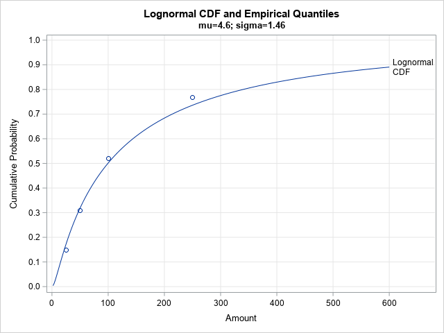
The fit isn't terrible. The distribution passes close to the other empirical quantiles, but perhaps we can do better? An alternative method of fitting the parameters is shown in the next section.

A least squares fit for the quantiles

Instead of using only two of the published sample statistics to fit the lognormal distribution, what if we tried to use all four published quantiles? We could try to minimize the sum of the squared residuals between the empirical cumulative probabilities and the CDF of the fitted lognormal distribution. I have previously shown how to perform this analysis in SAS by using PROC NLIN:

/* Can we obtain a better fit if we use all four quantiles to fit the distribution? */
/* https://blogs.sas.com/content/iml/2018/03/07/fit-distribution-matching-quantile.html */
/* least squares fit of parameters */
proc nlin data=Quantiles /* sometimes the NOHALVE option is useful */
          outest=PE(where=(_TYPE_="FINAL"));
   parms mu 4.6 sigma 1.46;
   bounds 0 < sigma;
   model ECDF = cdf("Lognormal", Amount, mu, sigma);
run;
 
proc print data=PE noobs;
   var mu sigma;
run;
 
data LogNormalCDF2;
mu = 4.55223; sigma = 1.29609;
do Amount = 2 to 600 by 2;
   LNCDF = cdf("Lognormal", Amount, mu, sigma);
   output;
end;
 
data All2;
   set LogNormalCDF2 Quantiles;
run;
 
title "Lognormal CDF and Empirical Quantiles";
title2 "mu=4.55; sigma=1.30";
proc sgplot data=All2 noautolegend;
   series x=Amount y=LNCDF / curvelabel='Lognormal/CDF' splitchar='/' splitjustify=left;
   scatter x=Amount y=ECDF;
   xaxis grid;
   yaxis grid values=(0 to 1 by 0.1) max=1 label="Cumulative Probability";
run;

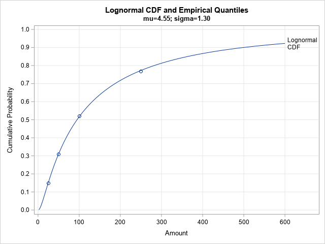
By using PROC NLIN to minimize the squared residuals, the CDF of the LN(4.55, 1.30) distribution is very close to the empirical CDF (ECDF). This might be a better model for the (unknown) data than the first model.

Flexible distributions

The lognormal distribution seems to fit the summary statistics in this example. However, it only has two parameters. There are other distributions that have more parameters and are more flexible. One flexible distribution is the metalog distribution, which is ideal for fitting a distribution to published sample quantiles. Similar to the previous example, you fit a metalog distribution by minimizing the sum of the squared residuals. But for the metalog distribution, you minimize the squared residuals between the observed quantiles and the distribution's quantiles. (Recall that the quantile function is the inverse CDF.)

You can use the metalog distribution in the SAS IML language by downloading SAS IML modules directly from a GitHub site. The following statements assume that you have downloaded the SAS IML modules from GitHub and have used the %INCLUDE statement to store the modules.

It is simple to fit a metalog distribution to empirical quantiles. The process is exactly the same as shown in the article, "Fitting a distribution to an expert's opinion." For these data, you have four empirical quantiles, so the order of the metalog distribution cannot exceed 4. The following example fits a fourth-order metalog model and plots the CDF and the empirical statistics. Although you can fit an unbounded metalog model, the following program fits a bounded distribution with support on the interval [$2, $30,000].

proc iml;
/* This LOAD statement assumes that the metalog functions are defined as in  Appendix A of the documentation.
   See the MetalogDoc.pdf file at https://github.com/sassoftware/sas-iml-packages/tree/main/Metalog */
load module=_all_;
use Quantiles;
   read all var {'Amount' 'ECDF'};
close;
 
bounds = {2 30000};       /* bounded on [2, 30k] */
order = 4;                /* must be <= num data */
MLObj = ML_CreateFromCDF(Amount, ECDF, order, bounds);
 
p = do(0, 0.9, 0.01);
title "Metalog Distribution for Empirical Quantiles";
call ML_PlotECDF(MLObj, p);

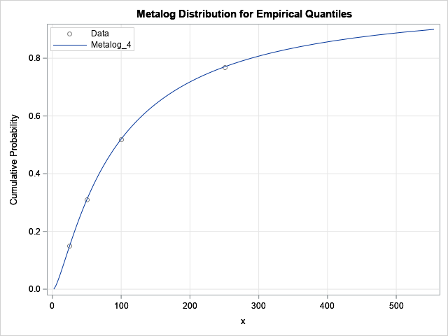
The graph indicates that the metalog distribution fits the empirical quantiles extremely well.

One application of fitting a distribution to the descriptive statistics is simulating example data. You can use the ML_RAND function in the Metalog package to simulate a random sample from a metalog distribution. The following statements simulate 1,000 random variates and draw a histogram so that you can see the distribution of the sample:

call randseed(123, 1);
n = 1000;     
Amount = ML_Rand(MLObj, n);
Amount = round(Amount, 0.01);   /* round to nearest $0.01 */
 
title "Simulated Distribution of Check Amounts";
title2 "Amount ~ Metalog(4, [2,30000])";
title3 "Amount < $1000";
call histogram(Amount[loc(Amount<1000)] ) rebin={12.5, 25};

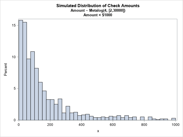
The histogram shows the distribution of the random sample for check amounts less than $1,000. You can see that the distribution has a long tail. The sample mean is $284.20; the sample median is $103.65. The largest check in this sample (not shown) is $14,889.20.

Summary

This article discusses three ways to fit a distribution to published statistics such as means and quantiles. First, we fit the two parameters in a lognormal distribution by using the sample mean and median. The resulting distribution did not fit the other sample quantiles very well. Next, we used PROC NLIN to find parameters for which the CDF and the ECDF are closest in a least-squares sense. Lastly, we used the metalog distribution, which is a flexible distribution, to obtain a least-squares fit to the empirical quantiles. You can use the metalog distribution to fit data distributions that do not appear to come from a "named" family. You can always simulate data from a metalog distribution, not matter how complicated the model is.