Does anyone write paper checks anymore? According to researchers at the Federal Reserve Bank of Atlanta (Greene, et al., 2020), the use of paper checks has declined 63% among US consumers since the year 2000. The researchers surveyed more than 3,000 consumers in 2017-2018 and discovered that only 7% of financial transactions used paper checks. Furthermore, they compiled the following statistics:

• On average, the consumer in their study wrote 3.3 checks per month or 39.6 checks per year.
• The average check value was $291.
• The median check value was $100.
• Among the data, the minimum check value was $2, and the maximum was $30,000.
• Older, lower-income, white people are more likely to use paper checks than other demographic groups.

Notice that these statistics describe two different random variables: The number of checks written by each individual, and the amount of the check. When I see a study like this, I wonder about the distributions of each random variable, and how I might simulate the data.

This article discusses how to simulate these data in SAS. For each individual, you can simulate the number of checks that he writes in a given time period. For each check, you can simulate the amount. To simplify the discussion, we ignore covariates such as age, income, and race, which might affect the number of checks and their amounts. Instead, we assume a homogeneous check-writing population.

Simulate the number of events and the amount

It is common to encounter data for which the frequency and size of an event are both important. For example, in longitudinal clinical studies, each subject has a certain number of visits to the clinic and for each visit has one or more measurements such as blood pressure, cholesterol, and so forth. In weight loss studies, participants record the number of times that they exercised, as well as a quantity (time or calories) related to the amount that they exercised. In all these cases, you can model the number of events and the size of each event.

Without access to the actual data, you must make a few assumptions about the distribution of the two random variables. Both assumptions could be checked against actual data, if you have any.

• The number of checks is distributed as a Poisson random variable with an expected value of 39.6 checks per year.
• The amount of the check is a positive skewed distribution with a median value of $100 and an average value of $291. There are infinitely many distributions that you could use, but let's use the lognormal distribution because it is a familiar distribution that models a positive quantity.

The main reason I chose a two-parameter lognormal distribution is because you can explicitly find the values of the parameters for which the distribution has a specified median and mean. (I have previously used this trick to choose parameter values that have a specified mean and variance.) As indicated in the Wikipedia article, the lognormal LN(μ, σ) distribution has median exp(μ) and mean exp(μ + σ²/2). By setting the median and mean equal to the corresponding sample statistics (100 and 291, respectively) you can solve for the lognormal parameter values. You obtain μ = 4.6 and σ = 1.46. The following SAS DATA step simulates writing checks for 20 individuals over the course of one year by using the Poisson(39.6) and the LN(4.6, 1.46) distributions. The call to PROC MEANS summarizes the statistics for the simulated data.

%let numSubjects = 20;
data Checks;
call streaminit(123);
mu = 4.6; sigma = 1.46;
do ID = 1 to &numSubjects;
   numChecks = rand("Poisson", 3.3 * 12);  /* avg 3.3 checks per month */
   do checkNum = 1 to numChecks;
      Amount = round(rand("Lognormal", mu, sigma), 0.01);  /* round to nearest $0.01 */
      output;
   end;
end;
keep ID numChecks checkNum Amount;
run;
 
proc means data=Checks Min Mean Median Max ndec=2;
   var numChecks Amount;
run;

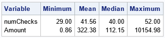
Recall that the Poisson distribution returns an integer, so the number of checks is always an integer. In contrast, I used the ROUND function to round the amount of the check to the nearest $0.01. The table shows that the number of checks ranges from a low of 29 to a high of 52, with a median value of 40. The amount of the checks ranges from $0.86 to $10,154.98. These statistics are comparable to the statistics in the Federal Reserve paper.

You can draw histograms of the number of checks and the amounts to visualize the distributions of those quantities. Or, you can look at how these quantities vary across the 20 subjects. The following graph creates a box plot for each subject.

title "Simulated Distribution of Check Amounts per Subject";
title2 "Graph Truncated at Amount = $1000";
proc sgplot data=Checks;
   vbox Amount / category=ID;
   yaxis grid max=1000;
run;

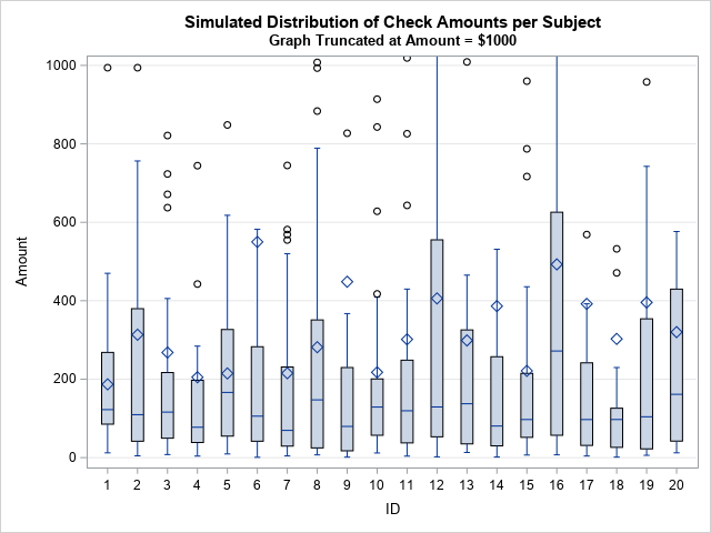
Each box shows the quartiles for the amounts. The horizontal line in the box visualizes the median check amount whereas the diamond marker shows the mean amount. You can see that the medians are close to $100 (the population median) whereas the means are close to $291 (the population mean).

Summary

This article describes how to simulate data for a common situation. In some studies, each subject experiences a random number of events. Associated with each event is one or more measurements. In this article, I used a Poisson distribution to simulate the number of paper checks (the event) written by each subject. I then used a lognormal distribution to model the amount of each check. Both distributions were chosen for their convenience and because they are easily fit by using the descriptive statistics mentioned in a journal article. If you have access to raw data, you can make a more informed choice about the models that you use in a simulation study.

The choice of a lognormal distribution is a big assumption. Perhaps there is a more principled way to choose a distribution that models the check amounts by using the information in the Federal Reserve paper? I pursue that question in a subsequent article.