 FINALLY…the simplest ESTIMATE statements to write are for continuous variables not involved in interactions or higher order terms.
Consider a data set containing the 2004 SAT scores for each of the 50 states. The file includes the combined math and verbal SAT scores (TOTAL), the state (STATE) and the percent of students participating in the test (PARTRATE). Suppose you assume a regression model to predict SAT scores as a linear function of the percentage of students in the state taking the test. The syntax for getting the estimated change in the score for a 20% increase in students taking the exam would be EASY for the following model!
proc glm data=sat2004;
model total=partrate;
ESTIMATE 'SAT Change for 20% Higher PartRate' partrate 20;
run;quit;
From the following output, our model estimates that a 20% increase in participation rate results in almost a 40 point drop in the average combined SAT score (with the standard error as shown).
Standard
Parameter Estimate Error t Value Pr > |t|
SAT Change for 20% Higher PartRate -39.6613349 3.11418443 -12.74 <.0001
However, it's best not to assume a linear model without first exploring the data. Let's create a scatter plot of the data using PROC SGPLOT and use the LOESS statement to detect potential trends in the data:
proc sgplot data=sat2004;
scatter y=total x=partrate;
loess y=total x=partrate / nomarkers;
title 'Explore SAT Scores Dataset';
run;
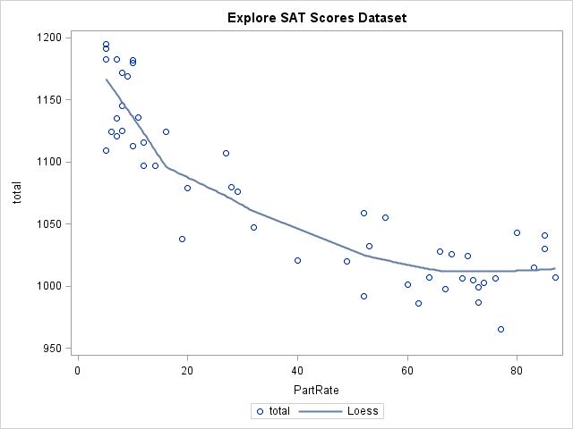
As the percent of students taking the tests increases (PartRate), the total score on the SAT decreases, but not in a linear fashion. Above about a 60% participation rate, the plot for the total score appears flat. To capture the curvature, include both quadratic and linear terms of participation rate in the model:
proc glm data=sat2004;
model total=partrate partrate*partrate;
title 'Quadratic Model';
run;
The output from the Parameter Estimates table indicates that both the linear and quadratic terms are significant in the model:
Parameter Estimate Standard Error t Value Pr > |t|
Intercept 1185.715281 9.01781421 131.49 <.0001
PartRate -5.215672 0.62285184 -8.37 <.0001
PartRate*PartRate 0.038318 0.00723291 5.30 <.0001
ESTIMATE statements can answer the question "how much does the predicted SAT score change when the number of students taking the test increases by XX%?" for this model. However, since we don't have a linear relationship, we have to specify where on the curve we would like to estimate our change.
For example, look below at the estimated total scores when 20%, 40%, 60%, and 80% of students in a state take the exam. This is another type of ESTIMATE statement—one where you are asking for an estimate at a specific value of your predictor variable, rather than asking for a comparison. Notice that the intercept must be included with a coefficient of 1 for this type of ESTIMATE statement. (The ODS SELECT statement limits the output to the results of the ESTIMATE statement only.)
ods select 'Estimates';
proc glm data=sat2004;
model total=partrate partrate*partrate;
ESTIMATE '20%' intercept 1 partrate 20 partrate*partrate 400;
ESTIMATE '40%' intercept 1 partrate 40 partrate*partrate 1600;
ESTIMATE '60%' intercept 1 partrate 60 partrate*partrate 3600;
ESTIMATE '80%' intercept 1 partrate 80 partrate*partrate 6400;
title 'Estimates from Quadratic Model';
run;
quit;
In the code above, notice that in the estimate statement at 20% participation, the coefficient of the linear term is 20, but the coefficient of the quadratic term is 202, or 400. Similarly, for the estimate statement at 40% participation, the coefficients are 40 and 402 (1600), at 60% participation they are 60 and 602 (3600), and at 80% they are 80 and 802 (6400).
The output below indicates that the estimated total scores are approximately 1097 at 20% participation, 1039 at 40% participation, 1011 at 60%, and 1014 at 80% (with standard errors as shown).
Parameter Estimate Standard Error t Value Pr > |t|
20% 1096.72907 5.20224622 210.82 <.0001
40% 1038.39733 7.26081186 143.01 <.0001
60% 1010.72006 5.99461482 168.60 <.0001
80% 1013.69726 7.43284299 136.38 <.0001
While the participation rate is increasing at a constant rate of 20%, the estimated scores decrease, but not at a constant rate. So…what coefficients would you use to get an estimated change in total SAT score for a change of 20% in the participation rate?
For all instances of a 20% increase, the linear coefficient will be 20. Since the relationship is not linear, the coefficients for the quadratic term depend on where you are measuring the change. You can obtain the correct coefficient for the quadratic term by taking the difference of the quadratic coefficients (as found in the previous ESTIMATE statements) for our starting and ending participation rates. For example,
- an increase from 20% to 40% participation rate would have a quadratic coefficient of 1200 (1600-400);
- an increase from 40% to 60% would have a quadratic coefficient of 2000 (3600-1600);
- an increase of 60% to 80% would have a quadratic coefficient of 2800 (6400-3600).
The syntax for the ESTIMATE statements would be:
proc glm data=sat2004;
model total=partrate partrate*partrate;
ESTIMATE 'Increase from 20% to 40%' partrate 20 partrate*partrate 1200;
ESTIMATE 'Increase from 40% to 60%' partrate 20 partrate*partrate 2000;
ESTIMATE 'Increase from 60% to 80%' partrate 20 partrate*partrate 2800;
title 'Estimates for 20% Increases from 20%, 40% and 60% PartRate';
run;
quit;
Parameter Estimate Standard Error t Value Pr > |t|
Increase from 20% to 40% -58.3317408 4.32058228 -13.50 <.0001
Increase from 40% to 60% -27.6772689 3.37111967 -8.21 <.0001
Increase from 60% to 80% 2.9772030 8.42760869 0.35 0.7254
The estimated change in SAT scores is
- approximately a 58 point decrease (standard error 4.3) when increasing participation rates from 20% to 40%;
- approximately a 28 point decrease (standard error of 3.4) when increasing participation rates from 40% to 60%;
- not significantly different from 0 when increasing participation rates from 60% to 80%.
While linear models certainly have the easiest ESTIMATE statements, getting the correct estimates depends first on getting the appropriate model. By exploring the data before building the model and writing your ESTIMATE statements, you can ensure meaningful results.
This is our last installment on ESTIMATE statements, so feel free to suggest topics for future blogs.