Visualize the placement of knots for regression splines

Splines are useful tools for fitting regression models to data. A spline replaces a single variable (call it X) with several other variables, which are a spline basis for X. When using a spline basis, the shape and location of the basis functions depend on the placement of knots. Knots are breakpoints that partition the range of a variable into subintervals. The regression model can fit the behavior of the data separately on each subinterval.

This article explains, compares, and visualizes common knot-placement schemes for regression splines.

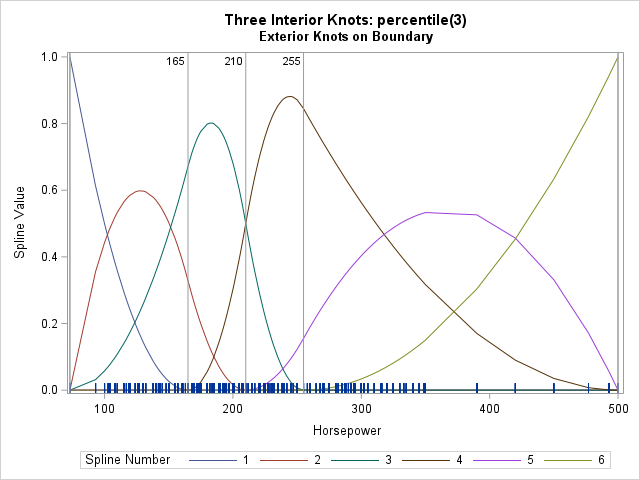
Previous articles about regression splines have visualized natural cubic splines and truncated power functions (TPF). This article focuses on B-splines. B-splines not only require placing "internal" knots which are within the range of the data for X, but also use "external" or "boundary" knots. Consequently, this article also discusses how the placement of external knots affects the spline basis. A typical visualization is shown to the right for a B-spline basis. The vertical reference lines indicate the locations of knots.

For previous articles about splines, see

"Regression with restricted cubic splines in SAS": How to use the EFFECT statement in SAS to define and use splines in regression models. This article discusses the KNOTMETHOD= option, which enables you to specify the placement of the knots.
"Visualize a regression with splines": How to visualize the spline basis and interpret the parameters in a regression model that includes splines.

Why use splines for regression?

Why are splines useful in regression modelling? Briefly, splines enable you to use linear regression models to fit data that have local or even nonlinear effects. In an elementary linear model, you model the response variable (Y) as a linear combination of one or more independent variables. In the simplest case of one independent variable, the model is Y = b0 + b1*X1 + error. This model is only reasonable if Y and X are linearly related across the entire range of X, which is not always true. Splines enable you to fit a piecewise-linear models where the model changes on various subintervals of the X range. The knots define the subintervals. You can also use knots and splines to fit a piecewise-polynomial model. This is shown in subsequent sections. It is possible because the basis functions for B-splines (and other polynomial-based splines) are formed by piecewise polynomials of degree d that are joined together so that they are continuously differentiable up to order d-1.

Sample data

I'll demonstrate the knot placement and the spline visualization by using the Horsepower variable in the SasHelp.Cars data set, which has 428 observations. In this article, the phrase "the X variable" refers to the Horsepower variable. So that you can easily run the examples on your own data, I have put the name of the data set and the name of the variable into macro variables (DSName and XVar, respectively). By modifying those two macro variables, the code in this article should work for any data set and any numerical variable.

The following SAS statements define the data and the macro variables:

/* example data */
data Have;
set sashelp.cars;
keep Horsepower;
run;
 
/* define these macro variables to point to your data set and numerical variable */
%let DSName = Have;
%let XVar = Horsepower;
 
/* you should not have to modify any code below this line */
data SplDS / view=SplDS;
   set &DSName;
   _Fake = 0;    /* add fake variable for the MODEL statement in PROC GLMMIX */
run;

The code creates a DATA step view that adds a dummy variable (_Fake) to the data set. You can use PROC MEANS to obtain the five-number summary of the data:

proc means data=SplDS min Q1 median Q3 max ndec=0;
   var &XVar;
run;

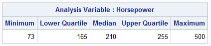
The range of the data is [73, 500].

Overview of knot placement methods

In SAS regression procedures, the location of knots is determined by the KNOTMETHOD= option on the EFEFCT statement. In this article, the examples always use the BASIS=BSPLINE and DEGREE=2 options. In practice, many people use DEGREE=3, which results in more basis functions.

The knot placement options are as follows:

PERCENTILES(n) and PERCENTILELIST(percentile-list): The knot locations are placed at percentiles of the X variable. For a B-spline basis, the external knots are placed at min(X) and max(X).
EQUAL(n): The knot locations are placed at n evenly spaced points inside the interval [min(X), max(X)]. For a B-spline basis, the external knots are placed at evenly spaced points less than or equal to min(X) and greater or equal to max(X). The distance between all knots (exterior and interior) is the same.
RANGEFRACTIONS(fraction-list): If the fraction list is (f1, f2, f3,...), the knot locations are placed at min(X) + (max(X)-min(X))*f_i, where 0 < f_i ≤ 1. For a B-spline basis, the external knots are placed at min(X) and max(X).
LIST(number-list) and LISTWITHBOUNDARY(number-list): The knot locations are placed at specified locations in data coordinates. For a B-spline basis, the LIST option places external knots at min(X) and max(X). The LISTWITHBOUNDARY option enables you to specify the location of the internal and external knots.

The PERCENTILES and PERCENTILELIST methods

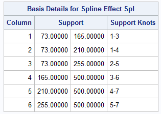
The knot locations are placed at percentiles of the X variable. For a B-spline basis, the external knots are placed at min(X) and max(X). The following call to PROC GLMIMMIX includes an EFFECT statement. The KNOTMETHOD= option specifies the PERCENTILES(3) option, which places knots at the 25th, 50th, and 75th percentile of the X variable. The OUTDESIGN= option on the PROC GLMMIX statement creates a SAS data set that contains the spline bases evaluated at the values of the X variable. For a DEGREE=2 basis, the columns of the data set are named Spl1--Spl6. The NOINT option on the MODEL statement prevents the OUTDESIGN= data set from containing a constant column of 1s.

/* PERCENTILES(n) specifies the locations for internal knots as n even percentiles of the data. 
   For a B-spline basis, the extremes of the data are used as boundary knots.
*/
proc glimmix data=SplDS NOFIT
             outdesign(names X=Spl)=Pctl_BSpl;
   effect Spl=spline( &XVar / basis=BSpline details degree=2
                      knotmethod=percentiles(3) ); /* <== KNOTMETHOD */
   model _Fake = Spl / NOINT;
   ods select SplineKnots BSplineDetails;
   ods output SplineKnots=KnotPositions;
run;

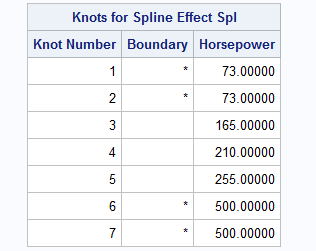
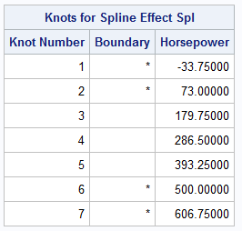
The ODS SELECT statement selects two output tables, which are shown above. The SplineKnots table provides information about the placement of knots. For the PERCENTILES(3) method, there are d knots placed at the minimum value of the X variable, 3 interior knots placed at the 25th, 50th, and 75th percentiles of the X variable, and d knots placed at the maximum value of the X variable. The exterior or boundary knots are indicated by an asterisk. Notice that it is mathematically acceptable to stack two or more knots at the same position.

The BSplineDetails was created by using the DETAILS option on the EFFECT statement. It tells you that the basis consists of 6 spline functions. The first basis function has support (that is, nonzero values) on the interval defined by the first three knots, which is [min(X), 25_th_Pctl]. The second basis function has support on the interval defined by the knots 1-4, which is [min(X), 50_th_Pctl]. This information continues until the sixth basis function, which has support on the interval defined by the knots 5-7, which is [75_th_Pctl, max(X)].

You can visualize the spline basis on the range of the X variable. If X has widely spaced values, the splines might look "chunky" when evaluated at the values of X. However, the basis functions are piecewise polynomials in the intervals between the knots, so they are continuous and smooth. For a spline basis of degree d, the basis functions are continuously differentiable d-1 times at the knot locations. The following statements create the visualization by using the %SplineViz macro, which is defined in the Appendix.

title "Three Interior Knots: percentile(3)";
title2 "Exterior Knots on Boundary";
%SplineViz( Pctl_Knots );

The six spline basis functions are shown. The vertical lines indicate the placement of knots. The knots define subintervals on which the splines are defined. The splines look smooth on the left because X has many unique values there. The splines look "chunky" on the right because there are only a few unique values of X that are greater than 350.

The shape of the interior splines might remind you of probability distributions. Some are roughly "bell-shaped" whereas others are skewed. Because the exterior knots are clamped at the extremes of the data, the first and last spline functions look like truncated polynomials that have the values 0 and 1 at the endpoint of the subinterval on which they are defined.

The EQUAL method

The KNOTMETHOD=EQUAL(n) option is similar to the PERCENTILES(n) option, except the knot locations for EQUAL(n) are placed at n evenly spaced points inside the interval [min(X), max(X)]. For a B-spline basis, the external knots are also evenly spaced points. The leftmost knots are less than or equal to min(X); the rightmost knots are greater than or equal to max(X). The distance between all knots (exterior and interior) is the same.

For example, the following call to PROC GLIMMIX uses the EQUAL(3) option. Otherwise, the syntax to PROC GLIMMIX is unchanged.

/* EQUAL(n) specifies that n equally spaced knots be positioned between the 
   extremes of the data. For a B-spline basis, any needed boundary knots 
  continue to be equally spaced. You can use the DATABOUNDARY option to override this behavior.
*/
proc glimmix data=SplDS NOFIT
             outdesign(names X=Spl)=Equal_BSpl;
   effect Spl=spline( &XVar / details basis=BSpline degree=2
                              knotmethod=EQUAL(3) ); /* <== KNOTMETHOD */
   model _Fake = Spl / NOINT; 
   ods select SplineKnots;
   ods output SplineKnots=KnotPositions;
run;

The output shows that the knots are equally spaced. The distance between adjacent knots is Δx = 106.75. The exterior knots on the left are at min(X)-Δx and min(X). The interior knots are at min(X) + i*Δx for i=1,2,3. The exterior knots on the right are placed at max(X) and max(X)+Δx. The following statements visualize the spline basis for this set of knots:

title "Three Interior Knots: equal(3)";
title2 "Exterior Knots Are Equally Spaced";
%SplineViz( Equal_BSpl );

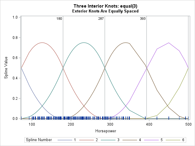
These basis functions are essentially identical, ignoring the "chunky" artifacts on the right. The functions differ by a shift.

The RANGEFRACTIONS method

The RANGEFRACTIONS method is similar to EQUAL method but enables you to set knots at unequal positions within the range of the X variable. If the fraction list is (f1, f2, f3,...), the knot locations are placed at min(X) + (max(X)-min(X))*f_i, where 0 < f_i ≤ 1. So, you can recreate the EQUAL(3) spacing by using RANGEFRACTIONS(0.25 0.5 0.75). If you want unequal spacing, you can use a syntax such as RANGEFRACTIONS(0.2 0.5 0.8) to position the knots at 20%, 50%, and 80% of the range.

For a B-spline basis, the RANGEFRACTIONS method places the external knots at min(X) and max(X). Let's place three interior knots at evenly spaced positions within the range but clamp the exterior knots at the extremes of the data. This will enable us to compare spline bases that differ only by the exterior knots:

/* RANGEFRACTIONS(fraction-list) specifies that internal knots be placed at each fraction of the range of X.
   For a B-spline basis, the data extremes are used as boundary knots.
*/
proc glimmix data=SplDS nofit
             outdesign(names X=Spl)=Range_BSpl;
   effect Spl =spline(&XVar / basis=BSpline details degree=2
                                  knotmethod=rangefractions(.25 .5 .75) );
   model _Fake = Spl / NOINT; 
   ods select SplineKnots;
   ods output SplineKnots=KnotPositions;
run;

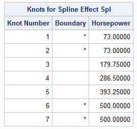
The output confirms that the interior knots are placed the same as for the EQUAL(3) option, but the exterior knots are clamped at the extreme values of the data. The following statement visualize the spline basis:

title "Three Interior Knots: rangefractions(.25 .5 .75)";
title2 "Exterior Knots Are Clamped at Min/Max";
%SplineViz( Range_BSpl );

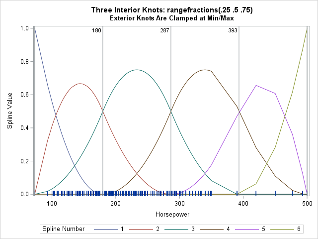
This spline basis differs from the EQUAL(3) basis, which was highly symmetric. Placing the exterior knots at the boundary of the data means that the range of the first and last spline is [0,1]. The interior splines are not the same size and shape. (Or, perhaps I should quip that they are KNOT the same shape!)

The LIST and LISTWITHBOUNDARY methods

The LIST and LISTBOUNDARY methods enable you to place the knots by using the data scale. I will not show an example. You merely list the data values at which you want the knots.

Summary

This article shows how to position knots for regression splines by using the KNOTMETHOD= option on the EFFECT statement, which is supported by many SAS regression procedures. You can use the OUTDESIGN= option on the PROC GLIMMIX statement to output the splines (evaluated at the data locations) to a data set. The output from PROC GLIMMIX includes the location of the knots. This article showed several common ways to place knots and, for each method, visualized the resulting set of spline basis functions.

Appendix: The SplineViz macro

The following macro visualizes the spline bases that are generated by each call to PROC GLMMIX. The name of the design matrix is passed in; inside the macro it is referred to as &DS. The columns for the spline basis are named Spl1, Spl2, Spl3, .... The positions of the knots are read from the KnotPositions data set, which was created from the ODS OUTPUT statement, which writes the SplineKnots table to a data set. The macro creates a series plot that shows the spline basis functions evaluated on the values of the data variable, X.

/* macro to visualize the spline bases that are generated by each call to PROC GLMMIX. 
   The original data should be sorted by the X variable.
   The name of the design matrix is passed in as &DS.
   The columns for the spline basis are named Spl1, Spl2, Spl3, ...
*/
%macro SplineViz( DS );
/* 1. Transpose design matrix from wide to long. The new variables are 
      SplNum : identifies the i_th basis function, i=1, 2, 3, ...
      Value  : the values of the X variable at which the i_th spline is evaluated
      Y      : the value of the i_th spline function evaluated at X
*/
data BSplineLong;
   set &DS;
   array basis Spl:;
   value = &XVar;
   do SplNum = 1 to dim(basis);
      Y = basis[SplNum];
      output;
   end;
   keep SplNum Value Y;
   label SplNum="Spline Number" Value="&XVar" Y="Spline Value";
run;
 
proc sort data=BSplineLong;
   by SplNum Value;
run;
/* add a label variable. You will need to change the format of these values
   if the scale of your data is larger or smaller than the example data.
*/
data SplineViz;
   set BSplineLong KnotPositions(keep=&XVar rename=(&XVar=KnotPos) );
   length KnotPosLabel $3;
   KnotPosLabel = putn(KnotPos, "3.0");
run;
 
proc sgplot data=SplineViz;
   series x=Value y=Y / group=SplNum nomissinggroup;
   fringe Value;
   refline KnotPos / axis=x labelloc=inside label=KnotPosLabel labelattrs=(size=8);
   yaxis max=1;     * for Viz, put all plots on same vertical scale;
run;
%mend;

Blogs