Most regression models try to model a response variable by using a smooth function of the explanatory variables. However, if the data are generated from some nonsmooth process, then it makes sense to use a regression function that is not smooth. A simple way to model a discontinuous process in SAS is to use spline effects and specify repeated value for the knots.

Discontinuous processes: More common than you might think

The classical ANOVA is one way to analyze data that are collected before and after a known event. For example, you might record gas mileage for a car before and after a tune-up. You might collect patient data before and after they undergo a medical or surgical treatment. You might have data about real estate prices before and after some natural disaster. In all these cases, you might suspect that the response changes abruptly because of the event.

To give a simple example, suppose that a driver records the fuel economy (in mile per gallon) for a car for 12 weeks. Because the car engine is coughing and knocking, the owner brings the car to a mechanic for maintenance. After the maintenance, the car seems to run better and he records the fuel economy for another six weeks. The hypothetical data are below:

data MPG;
input mpg @@;
week = _N_;
period = ifc(week > 12, "After ", "Before");
label mpg="Miles per Gallon";
datalines;
30.5 28.1 27.1 31.2 25.2 31.1 27.7 28.2 29.6 30.6 28.9 25.9 
30.6 33.0 31.2 29.7 32.7 31.1 
;

Notice that the data contains a binary indicator variable (period) that records whether the data are from before or after the tune-up. You can use PROC GLM to perform a simple ANOVA analysis to determine whether there was a significant change in the mean fuel economy after the maintenance. The following call to PROC GLM runs an ANOVA and indicates that the mean fuel economy is about 2.7 mpg better after the tune-up.

proc glm data=MPG plots=fitplot;
   class period / ref=first;
   model mpg = period /solution;
   output out=out predicted=Pred;
quit;

Graphically, this regression analysis is usually visualized by using two box plots. (PROC GLM creates the box plots automatically when ODS graphics are enabled.) However, because the independent variable is time, you could also use a series plot to show the observed data and the mean response before and after the maintenance. By using the GROUP= option on the SERIES statement, you can get two lines for the "before" and "after" time periods.

title "Piecewise Constant Regression with Jump Discontinuity";
proc sgplot data=Out;
   block x=week block=period / transparency=0.8;
   scatter x=week y=mpg / markerattrs=(symbol=CircleFilled color=black);
   series x=week y=pred / group=period lineattrs=(thickness=3) ;
run;

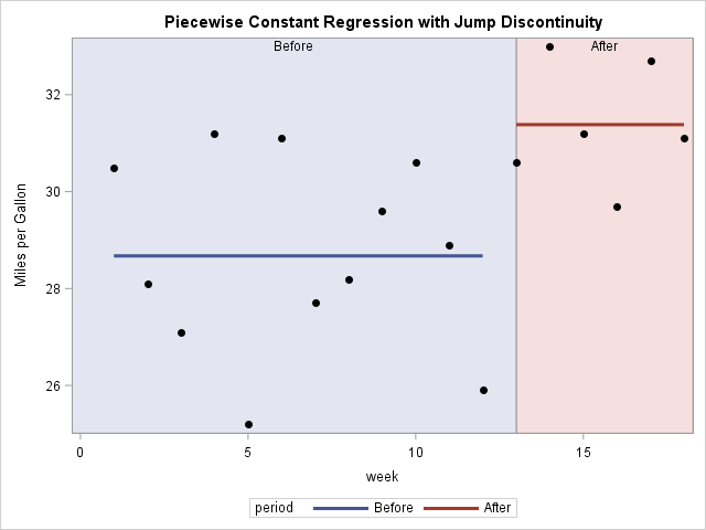
The graph shows that the model has a jump discontinuity at the time point at which the maintenance intervention occurred. If you include the WEEK variable in the analysis, you can model the response as a linear function of time, with a jump at the time of the tune-up.

All this is probably very familiar. However, did you know that you can use splines to model the data as a continuous function that has a kink or "corner" at the time of the maintenance event? You can use this feature when the model is continuous, but the slope changes at a known time.

Splines for nonsmooth models

Several SAS procedures support the EFFECT statement, which enables you to build spline effects. The paper "Rediscovering SAS/IML Software" (Wicklin 2010, p. 4) has an example where splines are used to construct a highly nonlinear curve for a scatter plot.

A spline effect is determined by the placement of certain points called "knots." Often knots are evenly spaced within the range of the explanatory variable, but the EFFECT statement supports many other ways to position the knots. In fact, the documentation for the EFFECT statement says: "If you remove the restriction that the knots of a spline must be distinct and allow repeated knots, then you can obtain functions with less smoothness and even discontinuities at the repeated knot location. For a spline of degree d and a repeated knot with multiplicity m ≤ d, the piecewise polynomials that join such a knot are required to have only d – m matching derivatives."

The degree of a linear regression is d=1, so if you specify a knot position once you obtain a piecewise linear function that contains a "kink" at the knot. The following call to PROC GLIMMIX demonstrates this technique. (I use GLIMMIX because neither PROC GLM nor PROC GENMOD support the EFFECT statement.) You can manually specify the position of knots by using the KNOTMETHOD=LIST(list) option on the EFFECT statement.

proc glimmix data=MPG;
   effect spl = spline(week / degree=1 knotmethod=list(1 13 18));     /* p-w linear */
   *effect spl = spline(week / degree=2 knotmethod=list(1 13 13 1); /*p-w quadratic */
   model mpg = spl / solution;  
   output out=out predicted=Pred;
quit;
 
title "Piecewise Linear Regression with Kink";
proc sgplot data=Out noautolegend;
   block x=week block=period / transparency=0.8;
   scatter x=week y=mpg / markerattrs=(symbol=CircleFilled color=black);
   series x=week y=pred / lineattrs=(thickness=3) ;
run;

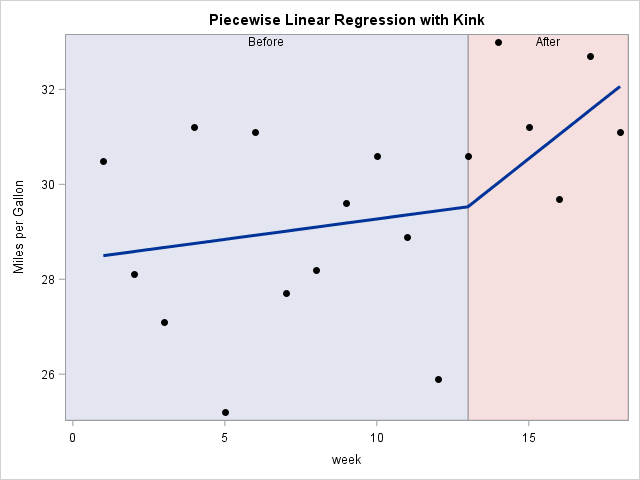
The graph shows that the model is piecewise linear, but that the slope of the model changes at week=13. In contrast, the second EFFECT statement in the PROC GLIMMIX code (which is commented out), specifies piecewise quadratic polynomials (d=2) and repeats the knot at week=13. That results in two quadratic models that give the same predicted value at week=13 but the model is not smooth at that location. Try it out!

If you are using a SAS procedure that does not support the EFFECT statement, you can use the GLMMIX procedure to output the dummy variables that are associated with the spline effects. A nice paper by David Pasta (2003) describes how to use dummy variables in a variety of models. The paper was written before the EFFECT statement; many of the ideas in the paper are easier to implement by using the EFFECT statement.

Lastly, the TRANSREG procedure in SAS supports spline effects but has its own syntax. See the TRANSREG documentation, which includes an example of repeating knots to build a regression model for discontinuous data.

Have you ever needed to construct a nonsmooth regression model? Tell your story by leaving a comment.