A segmented regression model is a piecewise regression model that has two or more sub-models, each defined on a separate domain for the explanatory variables. For simplicity, assume the model has one continuous explanatory variable, X. The simplest segmented regression model assumes that the response is modeled by one parametric model when X is less than some threshold value and by a different parametric model when X is greater than the threshold value. The threshold value is also called a breakpoint, a cutpoint, or a join point.

A previous article shows that for simple piecewise polynomial models, you can use the EFFECT statement in SAS regression procedures to use a spline to fit some segmented regression models. The method relies on two assumptions. First, it assumes that you know the location of the breakpoint. Second, it assumes that each model has the same parametric form on each interval. For example, the model might be piecewise constant, piecewise linear, or piecewise quadratic.

If you need to estimate the location of the breakpoint from the data, or if you are modeling the response differently on each segment, you cannot use a single spline effect. Instead, you need to use a SAS procedure such as PROC NLIN that enables you to specify the model on each segment and to estimate the breakpoint. For simplicity, this article shows how to estimate a model that is quadratic on the first segment and constant on the second segment. (This is called a plateau model.) The model also estimates the location of the breakpoint.

An example of a segmented model

A SAS customer recently asked about segmented models on the SAS Support Communities. Suppose that a surgeon wants to model how long it takes her to perform a certain procedure over time. When the surgeon first started performing the procedure, it took about 3 hours (180 minutes). As she refined her technique, that time decreased. The surgeon wants to predict how long this surgery now takes now, and she wants to estimate when the time reached its current plateau. The data are shown below and visualized in a scatter plot. The length of the procedure (in minutes) is recorded for 25 surgeries over a 16-month period.

data Have;
  input SurgeryNo Date :mmddyy10. duration @@;
  format Date mmddyy10.;
datalines;
1       3/20/2019       182   2       5/16/2019       150
3       5/30/2019       223   4       6/6/2019        142
5       6/11/2019       111   6       7/11/2019       164
7       7/26/2019        83   8       8/22/2019       144
9       8/29/2019       162  10       9/19/2019        83
11      10/10/2019       70  12       10/17/2019      114
13      10/31/2019      113  14       11/7/2019        97
15      11/21/2019       83  16       12/5/2019       111
17      12/5/2019        73  18       12/12/2019       87
19      12/19/2019       86  20       1/9/2020        102
21      1/16/2020       124  22       1/23/2020        95
23      1/30/2020       134  24       3/5/2020        121
25      6/4/2020         60
;
 
title "Time to Perform a Surgery";
proc sgplot data=Have;
  scatter x=Date y=Duration;
run;

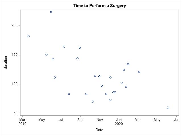
From the graph, it looks like the duration for the procedure decreased until maybe November or December 2019. The goal of a segmented model is to find the breakpoint and to model the duration before and after the breakpoint. For this purpose, you can use a segmented plateau model that is a quadratic model prior to the breakpoint and a constant model after the breakpoint.

Formulate a segmented regression model

A segmented plateau model is one of the examples in the PROC NLIN documentation. The documentation shows how to use constraints in the problem to eliminate one or more parameters. For example, a common assumption is that the two segments are joined smoothly at the breakpoint location, x0. If f(x) is the predictive model to the left of the breakpoint and g(x) is the model to the right, then continuity dictates that f(x0) = g(x0) and smoothness dictates that f`(x0) = g`(x0). In many cases (such as when the models are low-degree polynomials), the two constraints enable you to reparameterize the models to eliminate two of the parameters.

The PROC NLIN documentation shows the details. Suppose f(x) is a quadratic function f(x) = α + β x + γ x² and g(x) is a constant function g(x) = c. Then you can use the constraints to reparameterize the problem so that (α, β, γ) are free parameters, and the other two parameters are determined by the formulas:
x0 = -β / (2 γ)
c = α – β² / (4 γ)
You can use the ESTIMATE statement in PROC NLIN to obtain estimates and standard error for the x0 and c parameters.

Provide initial guesses for the parameters

As is often the case, the hard part is to guess initial values for the parameters. You must supply an initial guess on the PARMS statement in PROC NLIN. One way to create a guess is to use a related "reduced model" to provide the estimates. For example, you can use PROC GLM to fit a global quadratic model to the data, as follows:

/* rescale by using x="days since start" as the variable */
%let RefDate = '20MAR2019'd;
data New;
set Have;
rename duration=y;
x = date - &RefDate;  /* days since first record */
run;
 
proc glm data=New;
   model y = x x*x;
run;

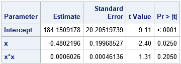
These parameter estimates are used in the next section to specify the initial parameter values for the segmented model.

Fit a segmented regression model in SAS

Recall that a SAS date is represented by the number of days since 01JAN1960. Thus, for these data, the Date values are approximately 22,000. Numerically speaking, it is often better to use smaller numbers in a regression problem, so I will rescale the explanatory variable to be the number of days since the first surgery. You can use the parameter estimates from the quadratic model as the initial values for the segmented model:

title 'Segmented Model with Plateau';
proc nlin data=New plots=fit noitprint;
   parms alpha=184 beta= -0.5 gamma= 0.001;
 
   x0 = -0.5*beta / gamma;
   if (x < x0) then
        mean = alpha + beta*x  + gamma*x*x;    /* quadratic model for x < x0 */
   else mean = alpha + beta*x0 + gamma*x0*x0;  /* constant model for x >= x0 */
   model y = mean;
 
   estimate 'plateau'    alpha + beta*x0 + gamma*x0*x0;
   estimate 'breakpoint' -0.5*beta / gamma;
   output out=NLinOut predicted=Pred L95M=Lower U95M=Upper;
   ods select ParameterEstimates AdditionalEstimates FitPlot;
run;

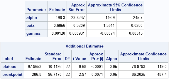
The output from PROC NLIN includes estimates for the quadratic regression coefficients and for the breakpoint and the plateau value. According to the second table, the surgeon can now perform this surgical procedure in about 98 minutes, on average. The 95% confidence interval [77, 119] suggests that the surgeon might want to schedule two hours for this procedure so that she is not late for her next appointment.

According to the estimate for the breakpoint (x0), she achieved her plateau after about 287 days of practice. However, the confidence interval is quite large, so there is considerable uncertainty in this estimate.

The output from PROC NLIN includes a plot that overlays the predictions on the observed data. However, that graph is in terms of the number of days since the first surgery. If you want to return to the original scale, you can graph the predicted values versus the Date. You can also add reference lines that indicate the plateau value and the estimated breakpoint, as follows:

/* convert x back to original scale (Date) */
data _NULL_;
   plateauDate = 287 + &RefDate;    /* translate back to Date scale */
   call symput('x0', plateauDate);  /* store breakpoint in macro variable */
   put plateauDate DATE10.;
run;
 
/* plot the predicted values and CLM on the original scale */
proc sgplot data=NLinOut noautolegend;
   band x=Date lower=Lower upper=Upper;
   refline 97.97  / axis=y label="Plateau"    labelpos=max;
   refline &x0 / axis=x label="01JAN2020" labelpos=max;
   scatter x=Date y=y;
   series  x=Date y=Pred;
   yaxis label='Duration';
run;

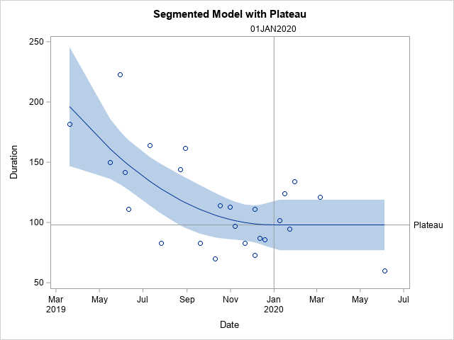
The graph shows the breakpoint estimate, which happens to be 01JAN2020. It also shows the variability in the data and the wide prediction limits.

Summary

This article shows how to fit a simple segmented model in SAS. The model has one breakpoint, which is estimated from the data. The model is quadratic before the breakpoint, constant after the breakpoint, and joins smoothly at the breakpoint. The constraints on continuity and smoothness reduce the problem from five parameters to three free parameters. The article shows how to use PROC NLIN in SAS to solve segmented models and how to visualize the result.

You can use a segmented model for many other data sets. For example, if you are a runner and routinely run a 5k distance, you can use a segmented model to monitor your times. Are your times decreasing, or did you reach a plateau? When did you reach the plateau?