This article describes how to obtain an initial guess for nonlinear regression models, especially nonlinear mixed models. The technique is to first fit a simpler fixed-effects model by replacing the random effects with their expected values. The parameter estimates for the fixed-effects model are often good initial guesses for the parameters in the full model.

Background: initial guesses for regression parameters

For linear regression models, you don't usually need to provide an initial guess for the parameters. Least squares methods directly solve for the parameter estimates by using the data. For iterative methods, such as logistic regression model, software usually starts with a pre-determined initial guess of the slope parameters and iteratively refine the guess by using an optimization technique. For example, PROC LOGISTIC in SAS begins by guessing that all slopes are zero. The "slopes all zero" model, which is better known as an intercept-only model, is a reduced model that is related to the full logistic model.

Several other regression procedures also fit a related (simpler) model and then use the estimates for the simpler model as an initial guess for the full model. For example, the "M method" in robust regression starts with a least squares solution and then iteratively refines the coefficients until a robust fit is obtained. Similarly, one way to fit a generalized linear mixed models is to first solve a linear mixed model and use those estimates as starting values for the generalized mixed model.

Fit a fixed-effect model to obtain estimates for a mixed model

The previous paragraphs named procedures that do not require the user to provide an initial guess for parameters. However, procedures such as PROC NLIN and PROC NLMIXED in SAS enable you to fit arbitrary nonlinear regression models. The cost for this generality is that the user must provide a good initial guess for the parameters.

This can be a challenge. To help, the NLIN and NLMIXED procedures enable you to specify a grid of initial values, which can be a valuable technique. For some maximum-likelihood estimates (MLE), you can use the method of moments to choose initial parameters. Although it is difficult to choose good initial parameters for a nonlinear mixed model, the following two-step process can be effective:

• Substitute the expected value for every random effect in the model. You obtain a fixed-effect model that is related to the original mixed model, but has fewer parameters. Estimate the parameters for the fixed-effect model. (Most random effects are assumed to be normally distributed with zero mean, so in practice you "drop" the random effects.)
• Use the estimates from the fixed-effect model as an initial guess for the full model. Hopefully, the initial guesses are close enough and the full model will converge quickly.

The following example shows how this two-step process works. The PROC NLMIXED documentation contains an example of data from an experiment that fed two different diets to pregnant rats and observed the survival of pups in the litters. The following SAS statements define the data and show the full nonlinear mixed model in the example:

data rats;
input trt $ m x @@;
x1 = (trt='c');
x2 = (trt='t');
litter = _n_;
datalines;
c 13 13   c 12 12   c  9  9   c  9  9   c  8  8   c  8  8   c 13 12   c 12 11
c 10  9   c 10  9   c  9  8   c 13 11   c  5  4   c  7  5   c 10  7   c 10  7
t 12 12   t 11 11   t 10 10   t  9  9   t 11 10   t 10  9   t 10  9   t  9  8
t  9  8   t  5  4   t  9  7   t  7  4   t 10  5   t  6  3   t 10  3   t  7  0
;
 
title "Full nonlinear mixed model";
proc nlmixed data=rats;
   parms  t1=2 t2=2 s1=1 s2=1;     /* <== documentation values. How to guess these??? */
   bounds s1 s2 > 0;
   eta = x1*t1 + x2*t2 + alpha;
   p   = probnorm(eta);
   model x ~ binomial(m,p);
   random alpha ~ normal(0,x1*s1*s1+x2*s2*s2) subject=litter;
run;

The model converges in about 10 iterations for the initial guesses on the PARMS statement. But if you deviate from those values, you might encounter problems where the model does not converge.

Fit a fixed-effect model to obtain initial estimates for the mixed model

The full mixed model has one random effect that involves two variance parameters, s1 and s2. If you replace the random effect with its expected value (0), you obtain the following two-parameter fixed-effect model:

title "Reduced model: Fixed effects only";
proc nlmixed data=rats;
   parms  t1=2 t2=2;
   eta = x1*t1 + x2*t2;
   p   = probnorm(eta);
   model x ~ binomial(m,p);
   ods output ParameterEstimates = FixedEstimates;
run;

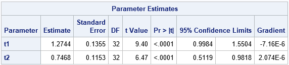
Notice that the estimates for t1 and t2 in the two-parameter model are close to the values in the full model. However, the two-parameter model is much easier to work with, and you can use grids and other visualization techniques to guide you in estimating the parameters. Notice that the estimates for t1 and t2 are written to a SAS data set called FixedEstimates. You can read those estimates on the PARMS statement by using a second call to PROC NLMIXED. This second call fits a four-parameter model, but the t1 and t2 parameters are hopefully good guesses so you can focus on finding good guesses for s1 and s2 in the second call.

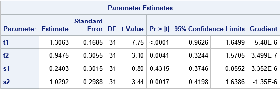
/* full random-effects model. The starting values for the fixed effects
   are the estimates from the fixed-effect-only model */
title "Full model: Estimates from a reduced model";
proc nlmixed data=rats;
   parms s1=0.1 s2=1 / data=FixedEstimates;   /* read in initial values for t1, t2 */
   bounds s1 s2 > 0;
   eta = x1*t1 + x2*t2 + alpha;
   p   = probnorm(eta);       /* standard normal quantile for eta */
   model x ~ binomial(m,p);
   random alpha ~ normal(0,x1*s1*s1+x2*s2*s2) subject=litter;
run;

Combining a grid search and a reduced (fixed-effect) model

You can combine the previous technique with a grid search for the random-effect parameters. You can use PROC TRANSPOSE to convert the FixedEstimates data set from long form (with the variables 'Parameter' and 'Estimate') to wide form (with variables 't1' and 't2'). You can then use a DATA step to add a grid of values for the s1 and s2 parameters that are used to estimate the random effect, as follows:

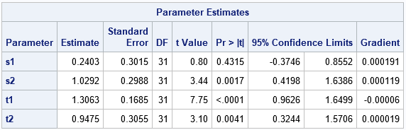
/* transpose fixed-effect estimates from long form to wide form */
proc transpose data=FixedEstimates(keep=Parameter Estimate) out=PE(drop=_NAME_);
   id Parameter;
   var Estimate;
run;
 
/* add grid of guesses for the parameters in the random effect */
data AllEstimates;
set PE;
do s1 = 0.5 to 1.5 by 0.5;     /* s1 in [0.5, 1.5] */
   do s2 = 0.5 to 2 by 0.5;    /* s2 in [0.5, 2.0] */
      output;
   end;
end;
run;
 
title "Full model: Estimates from a reduced model and from a grid search";
proc nlmixed data=rats;
   parms / data=AllEstimates;   /* use values from reduced model for t1, t2; grid for s1, s2  */
   bounds s1 s2 > 0;
   eta = x1*t1 + x2*t2 + alpha;
   p   = probnorm(eta);
   model x ~ binomial(m,p);
   random alpha ~ normal(0,x1*s1*s1+x2*s2*s2) subject=litter;
run;

The output is the same as for the initial model and is not shown.

In summary, you can often use a two-step process to help choose initial values for the parameters in a many-parameter mixed model. The first step is to estimate the parameters in a smaller and simpler fixed-effect model by replacing the random effects with their expected values. You can then use those fixed-effect estimates in the full model. You can combine this reduced-model technique with a grid search.

I do not have a reference for this technique. It appears to be "folklore" that "everybody knows," but I was unable to locate an example nor a proof that indicates the conditions under which this technique to work. If you know a good reference for this technique, please leave a comment.