SAS programmers sometimes ask, "How do I create a design matrix in SAS?" A design matrix is a numerical matrix that represents the explanatory variables in regression models. In simple models, the design matrix contains one column for each continuous variable and multiple columns (called dummy variables) for each classification variable.

I previously wrote about how to create dummy variables in SAS by using the GLMMOD procedure to create binary indicator variables for each categorical variable. But PROC GLMMOD is not the only way to generate design matrices in SAS. This article demonstrates four SAS procedures that create design matrices: GLMMOD, LOGISTIC, TRANSREG, and GLIMMIX. (Others include PROC CATMOD and PROC GLMSELECT.) Of the four, the LOGISTIC procedure is my favorite because it provides an easy-to-use syntax and supports various parameterizations for creating design matrices.

How categorical variables are represented in a design matrix in SAS

The CLASS statement in a SAS procedure specifies categorical variables that should be replaced by dummy variables when forming the design matrix. The process of forming columns in a design matrix is called parameterization or encoding. The three most popular parameterizations are the GLM encoding, the EFFECT encoding, and the REFERENCE encoding. For a detailed explanation of these encodings, see the section "Parameterization of Model Effects" in the SAS/STAT documentation. For applications and interpretation of different parameterizations, see Pasta (2005).

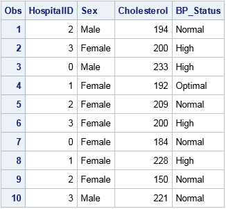
The following DATA step creates an example data set with 10 observations. It has three fixed effects: one continuous variable (Cholesterol) and two categorical variables. One categorical variable (Sex) has two levels and the other (BP_Status) has three levels. It also has a categorical variable (HospitalID) that will be used as a random effect.

data Patients;
   HospitalID = mod(_N_, 4);
   keep HospitalID Cholesterol Sex BP_Status;
   set sashelp.heart;
   if 18 <= _N_ <= 27;
run;
 
proc print; run;

PROC GLMMOD: Design matrices that use the GLM encoding

The simplest way to create dummy variables is by using the GLMMOD procedure, which can produce a basic design matrix with GLM encoding. The GLM encoding is a singular parameterization in which each categorical variable is represented by k binary variables, where k is the number of levels in the variable. There is also an intercept column that has all 1s. The GLMMOD procedure uses a syntax that is identical to the MODEL statement in PROC GLM, so it is very easy to create interaction effects. See my previous article for an example of how to use PROC GLMMOD to create a design matrix and how the singular parameterization affects parameter estimates in regression.

PROC LOGISTIC: Design matrices for any parameterization

You can also create a design matrix in SAS by using the LOGISTIC procedure. The PROC LOGISTIC statement supports an OUTDESIGNONLY option, which prevents the procedure from running the analysis. Instead, it only forms the design matrix and writes it to a data set. By default, PROC LOGISTIC uses the EFFECT encoding for classification variables, but you can use the PARAM= option on the CLASS statement to specify any parameterization.

A drawback of using PROC LOGISTIC is that you must supply a response variable on the MODEL statement, which might require you to run an extra DATA step. The following DATA step creates a view that contains a variable that has the constant value 0. This variable is used on the left-hand side of the MODEL statement in PROC LOGISTIC, but is dropped from the design matrix:

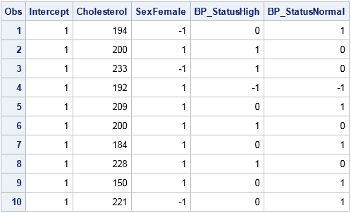
data Temp / view=Temp;
   set Patients;
   FakeY = 0;
run;
 
proc logistic data=Temp outdesign=EffectDesign(drop=FakeY) outdesignonly;
   class sex BP_Status / param=effect; /* also supports REFERENCE & GLM encoding */
   model FakeY = Cholesterol Sex BP_Status;
run;
 
proc print data=EffectDesign; run;

The design matrix shows the effect encoding, which uses –1 to indicate the reference level, which by default is the last level in alphabetical order. The name of a dummy variable is the concatenation of the original variable name and a level. For example, the Sex variable is replaced by the dummy variable named SexFemale, which has the value 1 to represent females and –1 to represent the reference level ("Male"). The BP_Status variable is replaced by two variables. The BP_StatusHigh variable contains 1 for patients that have high blood pressure, –1 for the reference level ("Optimal"), and 0 otherwise. Similarly, the BP_StatusNormal dummy variable has the value 1 for patients with normal blood pressure, –1 for the reference level ("Optimal"), and 0 otherwise.

The effect encoding produces k-1 columns for a categorical variable that has k levels. This results in a nonsingular design matrix.

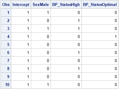
You can use the REF= option after each classification variable to specify the reference level. You can also use the PARAM= option on the CLASS statement to specify a different parameterization. For example, the following statements create a design matrix that uses the REFERENCE parameterization. The reference level for the Sex variable is set to "Female" and the reference level for the BP_Status variable is set to "Normal."

proc logistic data=Temp outdesign=RefDesign(drop=FakeY) outdesignonly;
   class sex(ref="Female") BP_Status(ref="Normal") / param=reference; 
   model FakeY = Sex BP_Status;
run;
 
proc print data=RefDesign; run;

Parameterizations affect the way that parameter estimates are interpreted in a regression analysis. For the reference encoding, parameter estimates of main effects indicate the difference of each level as compared to the effect of the reference level. For the effect encoding, the comparison is to the average effect over all levels.

PROC TRANSREG: Design matrices and a macro for variable names

Using PROC LOGISTIC is very flexible, but it has two drawbacks: You have to create a fake response variable, and you have to look at the output data set to discover the names of the dummy variables. In contrast, PROC TRANSREG does not require that you specify a response variable when you generate the design matrix. Furthermore, the procedure creates a macro variable (&_TRGIND, for "TRANSREG indicator" variables) that contains the names of the columns of the design matrix. Another nice feature is that the output data set contains the original variables, and you can use the ID variable to output additional variables.

However, the syntax for the TRANSREG procedure is different from most other SAS regression procedures. Instead of a CLASS statement, you specify classification effects in a CLASS() transformation list. By default, the procedure uses the REFERENCE parameterization; you can use the ZERO= option to control reference levels. The procedure also supports the GLM parameterization (via the ZERO=SUM option), the EFFECT parameterization (via the EFFECT option), and other options. The following statements show an example that generates a design matrix with the effect encoding:

proc transreg data=Patients design;
   model identity(Cholesterol) 
         class(Sex BP_Status / EFFECT zero="Female" "Normal");
   output out=B;
run;
 
proc print data=B; 
   var Intercept &_TrgInd; 
run;

The output is not shown because it is identical to the EffectDesign data set in the previous section. Notice that the output is displayed by using the &_TRGIND macro variable. For details about generating design matrices, see the TRANSREG documentation section "Using the DESIGN Output Option."

PROC GLIMMIX: Design matrices for fixed and random effects

PROC GLIMMIX enables you to construct two design matrices: one for the fixed effects and another for the random effects. The PROC GLIMMIX statement supports an OUTDESIGN= option that you can use to specify the output data set and a NOFIT option that ensures that the procedure will not try to fit the model.

The following statements create an output data set that contains two design matrices:

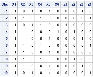
proc glimmix data=Patients outdesign(names novar)=MixedDesign nofit;
   class sex BP_Status HospitalID;
   model Cholesterol = Sex BP_Status;
   random HospitalID;
   ods select ColumnNames;
run;
 
proc print data=MixedDesign; run;

Dummy variables for the fixed effects are prefixed by "_X" and dummy variables for the random effects are prefixed by "_Z." Two additional tables (not shown) associate the levels of the original variables with the columns of the design matrices.

The GLIMMIX procedure uses only the GLM parameterization. Consequently, there is little advantage to using PROC GLIMMIX instead of PROC GLMMOD. You can generate the same designs by calling PROC GLMMOD twice, once for the fixed effects and once for the random effects.

Summary

In summary, SAS provides four procedures that you can use to generate design matrices for continuous variables, classification variables, and their interactions. The GLMMOD procedure is ideal for creating design matrices that use the GLM encoding. PROC LOGISTIC supports all encodings in SAS and provides an easy-to-use syntax for specifying interactions. PROC TRANSREG supports fewer parameterizations but does not require that you manufacture a response variable. Lastly, the GLIMMIX procedure produces design matrices for both fixed and random effects.

There are actually two other ways to create design matrices in SAS. For general linear models (like PROC GLM), you can use the OUTDESIGN option in the GLMSELECT procedure. If you need to use matrix computations, the SAS/IML procedure also supports creating design matrices.