A previous article discusses regression splines and how to use the EFFECT statement in SAS regression procedures to specify the location of knots for a regressor variable, X. Knots are breakpoints that partition the range of X into subintervals. The splines are defined on a set of adjacent subintervals. The EFFECT statement supports several common knot-placement methods including equally spaced knots, and knots placed at percentiles of the data. B-splines not only require placing "internal" knots within the range of the data but also use "external" or "boundary" knots. The EFFECT statement provides two methods for placing external knots: you can stack knots at the minimum and maximum value of X, or you can place the knots at equally spaced intervals outside of the data range.
The EFFECT statement provides a convenient way to specify knots and splines from within a SAS regression procedure. However, certain applications (such as simulation studies) require more control of knot placement. For these applications, SAS IML provides the BSPLINE function, which enables you to evaluate B-spline basis functions at a set of X values, given the knots. This article demonstrates the BSPLINE function and shows how to generate knots according to the common schemes that are supported by the EFFECT statement.
The example data
Unlike other statistical modeling methods, knots and splines can be defined without using any data. If you specify an interval, [a, b], and a set of knots, you can construct a B-spline basis on the interval. However, in practice, the interval is [min(X), max(X)] for some data variable, X. Furthermore, a common method to place the knots inside the interval is to use percentiles of the data. To accommodate these two facts, let's use the Horsepower variable in the Sashelp.cars data set as "X".
So that you can easily run the examples on your own data, I have put the name of the data set and the name of the variable into macro variables (DSName and XVar, respectively). By modifying those two macro variables, the code in this article should work for any data set and any numerical variable.
/* example data */ data Have; set sashelp.cars; keep Horsepower; run; /* define these macro variables to point to your data set and numerical variable */ %let DSName = Have; %let XVar = Horsepower; |
The BSPLINE function
PROC IML supports the BSPLINE function, which enables you to evaluate a B-spline basis function on an arbitrary set of X values.
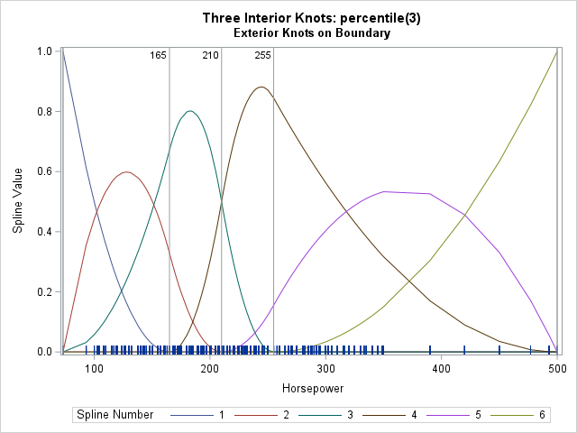
First, let me demonstrate that you don't need any data to generate a B-spline basis. For the Horsepower variable, X, min(X) = 73, max(X) = 500, and the 25th, 50th, and 75th percentiles of the data are 165, 210, 255. By using only these numbers, you can construct a B-spline basis on the interval [73, 500]. The following IML statements place internal knots at the values 165, 210, 255. There are two "clamped" boundary knots at the endpoints of the interval.
/* Use the BSPLINE function in PROC IML to reproduce an example from https://blogs.sas.com/content/iml/2026/04/22/viz-knots-splines.html which uses X=Horsepower variable from Sashelp.Cars */ proc iml; deg = 2; /* |-min(X)-|-25th 50th 75th Pctl -|-max(X)-| */ knots = {73, 73, 165, 210, 255, 500, 500}; t = T(do(73, 500, (500-73)/99)); /* evaluate at 100 points in range of X */ basis = bspline(t, deg, knots); /* 100x6 matrix. Columns are spline functions */ /* columns of BASIS are the splines evaluated at t */ title "Second Spline Basis"; call series( t, basis[,2] ) grid={x y} other="refline 165 210 255/axis=x;"; |
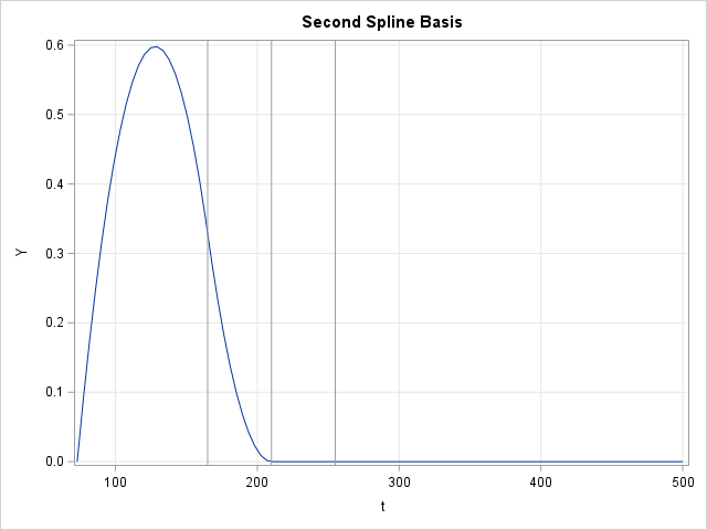
The BASIS variable is a matrix that has 100 rows and six columns. Each column is the result of evaluating a B-spline basis function at a set of evenly spaced values in the interval [73, 500]. The second basis function has support (that is, nonzero values) on the interval [73, 210]. The graph of that basis function is shown above.
The BASIS matrix contains the spline values in "wide form." If you want to visualize the basis by plotting all six functions on the same graph, you can use the WIDETOLONG function to reshape the data, then use the GROUP= option on the SERIES call to plot the functions, as follows:
/* if you want to plot all columns, convert wide to long and use the GROUP= option See https://blogs.sas.com/content/iml/2015/02/27/multiple-series-iml.html */ run WideToLong(tt, Value, Spline_Number, /* output (long) */ basis, t, "Spl1":"Spl6"); /* input (Basis is wide) */ title "All B-Splines (deg=2)"; call series(tt, Value) group=Spline_Number grid={X Y} other="refline 165 210 255/axis=x;" label={"&XVar" "Spline Value"}; |
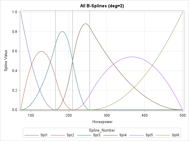
This graph shows the same B-spline basis as for the PERCENTILES(3) example in my previous article. The main difference is that the previous graph shows the splines evaluated at the observed values of X, whereas the graph in this article evaluates the splines on an evenly spaced grid of points. The second basis function is now displayed in a red color.
A SAS IML function for common knot-placement schemes
Although B-splines can be defined without any reference to data, in practice they are often used as regression splines. As such, the interval on which they are defined corresponds to the range of the X data. For some knot-placement schemes, the internal knots are placed at percentiles of the X variable. Furthermore, to create a design matrix for fitting a regression model, you must evaluate the splines at the observed values of X. So, in practice, it is useful to extract the knot positions from data.
As discussed in a previous article, the EFFECT statement in SAS regression procedures handles these details automatically. It is useful to define a SAS IML function that can generate the same knot-placement schemes that the EFFECT statement uses. The schemes that depend on the data are shown in the following table:
| Method | Parameter | Equivalent KNOTMETHOD= option | External Knots |
|---|---|---|---|
| "PCTL" | scalar n | PERCENTILES(n) | Boundary |
| "PCTL" | vector v | PERCENTILELIST(v), where 0 < v < 100 | Boundary |
| "EQUAL" | scalar n | EQUAL(n) | Evenly spaced |
| "RANGE" | vector v | RANGEFRACTIONS(v), where 0 < v < 1 | Boundary |
| "LIST" | vector v | LIST(v), where min(X) <= v <= max(X) | Boundary |
It is straightforward to define a SAS IML function that returns the same set of knots as the EFFECT statement. (You can skip the "LIST" method, which assumes that the user already knows the positions of the knots.) The following function shows one implementation, which uses separate helper functions for generating internal and external knots. You can test the function by loading the Horsepower variable and sending that data vector into the function, along with a parameter that specifies the number and location of knots. So that the main ideas are evident, this implementation does not perform any argument validation.
/* reproduce the knot-placement methods in the EFFECT statement: Method Parm Equivalent KNOTMETHOD= option External Knots ====== ======== ====================================== ============== "PCTL" scalar n PERCENTILES(n) Boundary "PCTL" vector v PERCENTILELIST(v), where 0 < v < 100 Boundary "EQUAL" scalar n EQUAL(n) Evenly spaced "RANGE" vector v RANGEFRACTIONS(v), where 0 < v < 1 Boundary */ start Knots(x, deg, method, parm); int_knots = Knots_Internal(x, method, parm); if upcase(method)="EQUAL" then do; delta = int_knots[2] - int_knots[1]; knots = Ext_Knots("EQUAL_L", deg, min(x), delta) // int_knots // Ext_Knots("EQUAL_R", deg, max(x), delta); end; else knots = Ext_Knots("BOUNDARY", deg, min(x)) // int_knots // Ext_Knots("BOUNDARY", deg, max(x)); return( knots ); finish; /* Helper: Function to create internal knots for B-splines. Valid methods are "PCTL", "EQUAL", or "RANGE". */ start Knots_Internal(x, method, _parm); parm = colvec(_parm); if upcase(method)="PCTL" then do; if nrow(parm)=1 then call qntl(knots, x, T(1:parm)/(parm+1)); /* PERCENTILES(n) */ else call qntl(knots, x, parm/100); /* PERCENTILELIST(v) */ end; else if upcase(method)="EQUAL" then knots = min(x) + range(x)*T(1:parm)/(parm+1); /* EQUAL(n) */ else if upcase(method)="RANGE" then knots = min(x) + range(x)*parm; /* RANGEFRACTIONS(v) */ else knots = .; /* unsupported method */ return( knots ); finish; /* Helper: Function to create external or boundary knots for B-splines. Valid methods are "BOUNDARY", "EQUAL_L", "EQUAL_R" */ start Ext_Knots(method, deg, value, delta=); if upcase(method)="BOUNDARY" then ext_knots = repeat(value, deg); if upcase(method)="EQUAL_L" then ext_knots = value - T((deg-1):0)*delta; if upcase(method)="EQUAL_R" then ext_knots = value + T(0:(deg-1))*delta; return( ext_knots ); finish; /* read in example data */ use &DSName; read all var "&XVar" into x; close; deg = 2; /* get knots for common placement schemes */ k_Pctl3 = Knots(x, deg, "PCTL", 3); k_PctlList = Knots(x, deg, "PCTL", {20, 50, 80}); k_eq3 = Knots(x, deg, "EQUAL", 3); k_RangeList = Knots(x, deg, "RANGE", {0.25, 0.50, 0.75}); /* display the results in a single table */ results = k_Pctl3 || k_PctlList || k_eq3 || k_RangeList; rowHeader = {'L Ext 1','L Ext 2','Int 1','Int 2','Int 3','R Ext 1','R Ext 2'}; colHeader = {'Pctl(3)','Pctl List','Equal(3)','Range List'}; print results[c=colHeader r=rowHeader L="Knot-Placement Methods"]; |
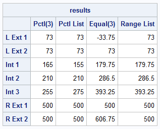
I reviewed the previous article and verified that these are the same knot positions that are generated by the EFFECT statement.
A design matrix for B-splines in SAS IML
If you plan to use B-splines in a regression model, you need to create the design matrix for the X variable. To generate a design matrix, you first specify a knot-placement scheme, which gives you a vector of knot locations. You can then call the BSPLINE function to produce the spline basis and evaluate the basis function at each observed value of X. The following statements show an example:
/* to generate a design matrix, first get the knots, then evaluate the splines on the X data */ knots = Knots(x, deg, "PCTL", {20, 50, 80}); basis = bspline(x, deg, knots); /* 428x6 matrix. Columns are spline functions */ |
The BASIS matrix is the design matrix for the splines. It does not include an intercept column. For a multivariable regression model, you would horizontally concatenate this design matrix with the data vectors or design matrices for additional regressors.
Visualize the B-spline basis
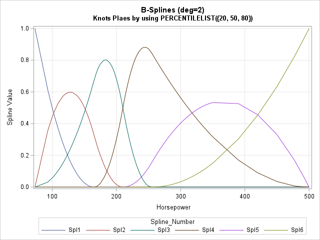
If you want to visualize the spline basis, you can add X to the design matrix, sort the columns, and then repeat the wide-to-long visualization from earlier in this article:
/* if you want to visualize, sort the data by the X variable, then convert wide to long */ M = x || basis; /* concatenate design matrix with X, then sort by X */ call sort(M, 1); t = M[,1]; basis = M[,2:ncol(M)]; run WideToLong(tt, Value, Spline_Number, /* output (long) */ basis, t, "Spl1":"Spl6"); /* input (Basis is wide) */ title "B-Splines (deg=2)"; title2 "Knots Placed by using PERCENTILELIST({20, 50, 80})"; call series(tt, Value) group=Spline_Number grid={X Y} label={"&XVar" "Spline Value"}; |
Summary
This article shows how to write a function in SAS IML that reproduces common knot-placement methods for B-splines. The B-splines use both Internal and external (or boundary) knots. Internal knots are placed within an interval, which is often the observed range of the data variable. Boundary knots are stacked at the endpoints of the interval. True external knots are placed outside the interval. After you generate the knots, you can then call the built-in BSPLINE function in IML to generate a spline design matrix.
Since most SAS regression procedures support the EFFECT statement, why would you want to generate knots and splines in IML? I can think of a few reasons:
- Varying the knot-placement scheme is useful for understanding whether the parameter estimates in a spline regression model are sensitive to the knot-placement method.
- If you want to generate your own knot-placement scheme, you can modify the IML functions in this article.
- By moving the generation of the spline design matrix into IML, you can easily run simulation studies and bootstrap analyses.
- B-splines are not the only type of spline. If you want to build a regression model that uses a new type of spline, you can reuse the standard knot-placement schemes for the new spline type.
