3 ways to estimate parameters when fitting a distribution to data

SAS provides procedures to fit common probability distributions to sample data. You can use PROC UNIVARIATE in Base SAS or PROC SEVERITY in SAS/ETS software to estimate the distribution parameters for approximately 20 common distributions, including normal, lognormal, beta, gamma, and Weibull.

Since there are infinitely many distributions, you may eventually need to fit a distribution that SAS does not natively support. There are three often-used methods for fitting the parameters of a distribution: the method of moments, the maximum likelihood optimization, and solving for the root of a complicated function. This article demonstrates all three methods by using the Gumbel distribution.

The Gumbel distribution

The Gumbel distribution is used to model extreme events, such as the maximum (or minimum) value of a random event, like the level of a river after rains. In SAS, the symbol μ is used for the location parameter and σ is used for the scale parameter. (Wikipedia and other sources use β for the scale parameter.) The PDF of the Gumbel distribution is given by
f(x; μ, σ) = exp(-z-exp(-z)) / σ, where z = (x - μ) / σ

In SAS, you can fit a Gumbel distribution to data by using the UNIVARIATE procedure, which uses maximum likelihood estimation (MLE) to estimate values for μ and σ.

Use PROC UNIVARIATE to fit a Gumbel model

The standard way to fit a Gumbel model to data is to use the HISTOGRAM statement in PROC UNIVARIATE. The documentation states that the HISTOGRAM statement "calculates maximum likelihood estimates for [the Gumbel]parameters." The following DATA step defines the maximum annual height of a river relative to a reference level. The call to PROC UNIVARIATE fits a Gumbel model to the data:

/* annual maximum height of river over 20-year period */
data Gumbel;
label y = "Maximum Height (cm)";
input y @@;
datalines;
46.8 48.0 50.1 51.7 50.5 49.9 51.5 50.4 47.9 49.3 
53.7 54.2 47.1 47.7 49.8 50.0 51.4 56.9 49.3 59.3 
;
 
/* Doc for PROC UNIVARIATE says "the procedure calculates maximum likelihood estimates" */
proc univariate data=Gumbel;
   var y;
   histogram y / gumbel;
   ods select Histogram ParameterEstimates;
run;

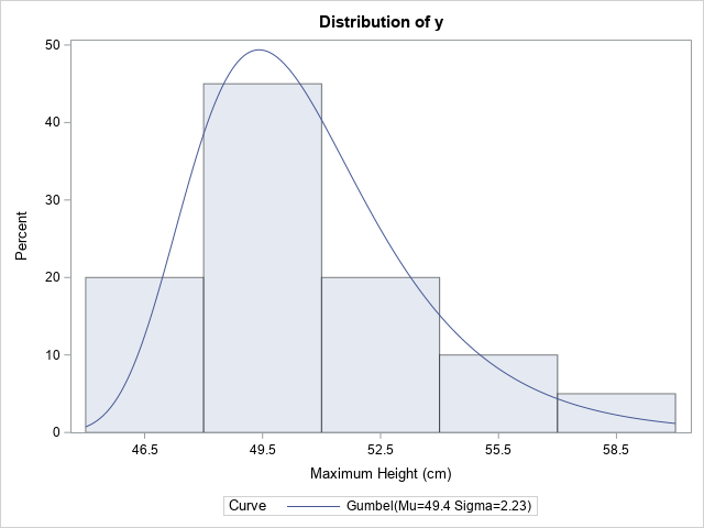
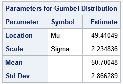
The histogram overlays the probability density function for the Gumbel(μ=49.4, σ=2.23) distribution. The MLE estimates are reported in the legend and in a separate ParameterEstimates table.

The remainder of this article implements three statistical methods to estimate parameters for a distribution. For each method, we will compare the answers that we get to the estimates that are produced by PROC UNIVARIATE.

The method of moments

The method of moments (MoM) is one of the earliest methods for fitting the parameters of a distribution. As opposed to MLE, the method of moments can often be carried out by hand. The idea is that you use calculus to express the first two moments of the distribution (the mean and the standard deviation) in terms of the parameters. The Wikipedia article for a distribution almost always shows these expressions. For example, the Wikipedia article for the Gumbel distribution states the following:
StdDev = π * σ / sqrt(6)
Mean = μ + σ * γ, where γ ≈ 0.577 is Euler's constant.

The method of moments is a "plug-in" method in which distributional parameters are replaced by their sample estimates. So, you replace the Mean and StdDev quantities by using the sample mean and the sample standard deviation. This results in two equations and two parameters (μ, σ), and you can invert these equations to solve for the unknowns:
σ = sqrt(6)*StdDev / π, where StdDev is now the SAMPLE standard deviation, and
μ = Mean – σ * γ, where Mean is the sample mean and σ is the estimate found in the previous statement.

Let's see the method of moments in action. You can use the CONSTANT function to obtain numerical values for π and γ. In Base SAS, you can use PROC MEANS to get the sample statistics and use the DATA step to apply the formulas to estimate σ and μ. However, since later sections of this article use PROC IML, let's solve the MoM problem in IML as well:

proc iml;
start Gumbel_MoM(y);
   pi = constant('pi');
   gamma = constant('Euler');
   sigma_MoM = sqrt(6)/pi * std(y);     /* use MEAN and STD to get sample moments */
   mu_MoM = mean(y) - gamma*sigma_MoM;
   return( mu_MoM // sigma_MoM );       /* return a 2x1 column vector */
finish;
/* read the sample data */
use Gumbel; read all var {'y'}; close;
 
/* Method 1: Method of Moments */
estimate_MoM = Gumbel_MoM(y);
print estimate_MoM[r={'Mu' 'Sigma'}];

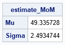
The MoM estimates differ from those provided by PROC UNIVARIATE, which uses MLE. However, for this data, the estimates are relatively close. That might not always be the case. One shortcoming of the method of moments is that the sample mean and the standard deviation are strongly influenced by outliers because they are not robust statistics. Nevertheless, the MoM is easy to implement and it is often used to provide an initial guess for the MLE optimization, as shown in the next section.

The traditional MLE

The traditional MLE method involves creating a log-likelihood function and summing the log-likelihoods over all observations. The SAS LOGPDF function does not support the Gumbel distribution, but you can derive it from the PDF function. The following SAS IML function takes a vector of parameters as an argument. It accesses the data by using a global variable, which I call G_Y because 'G_' is the prefix that I use for global variables.

/* Method 2: MLE using a direct LL function */ 
/* Log likelihood for Gumbel distribution:
       f(x) = (1/sigma) * exp(-(x-mu)/sigma) * exp(-exp(-(x-mu)/sigma))
   log f(x) = -log(sigma) - (x-mu)/sigma - exp(-(x-mu)/sigma)
            = -n*log(sigma) - sum(z) - sum(exp(-z)), where z=(x-mu)/sigma
*/
start Gumbel_LL(param) global(g_y);
   mu = param[1];
   sigma = param[2];
   z = (g_y-mu)/sigma;
   LL = -nrow(g_y) * log(sigma) - sum(z) - sum(exp(-z));
   return( LL );
finish;
 
g_y = y;        /* define the GLOBAL variable */
LL_MoM = Gumbel_LL(estimate_MoM);
print LL_MoM;

I strongly encourage you to always test and debug the objective function BEFORE using it in an optimization. After the function seems to work, you can use a nonlinear optimization method to find the parameters that maximize the log-likelihood. (Here, I use the quasi-Newton method, NLPQN.) For the Gumbel distribution, both parameters must be positive, so you should set boundary constraints. I set the lower bound on each variable to 1E-3 to bound the parameters away from zero. We need an initial guess for the optimization, so it is convenient to use the MoM estimates.

/* set constraint matrix, options, and initial guess for optimization */
con = { 1e-3 1e-3,     /* lower bounds: 0 < mu;  0 < sigma */
        .    .   };    /* upper bounds: None */
opt = {1,              /* find maximum of function   */
       2};             /* print some output      */
/* use estimate from method of moments as an initial guess */
call nlpqn(rc, estimate_MLE, "Gumbel_LL", estimate_MoM, opt, con); 
estimate_MLE = colvec(estimate_MLE);
print estimate_MLE[r={'Mu' 'Sigma'}];

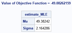
The output from the NLPQN subroutine includes the log-likelihood (LL) function value at the optimal parameter values. The LL value is larger than for the MoM estimates. The MLE estimates agree with the result of PROC UNIVARIATE.

Finding the MLE by solving for a root

Mathematically, the optimal value of the log-likelihood function, L(μ, σ), is the location for which the gradient of the function vanishes: $\frac{\partial L}{\partial \mu} = 0$ and $\frac{\partial L}{\partial \sigma} = 0$ . If you compute the derivative, you'll find that the MLE solution satisfies the following two equations:
$\begin{align*} \sigma &= \bar{x} - \frac{ \sum_{i=1}^n x_i \exp\left(-\frac{x_i}{\sigma}\right)} {\sum_{i=1}^n \exp\left(-\frac{x_i}{\sigma}\right) } \\ \mu &= -\sigma \log \left( \frac{1}{n} \sum_{i=1}^n \exp\left( -\frac{x_i}{\sigma} \right) \right) \end{align*}$

An important feature of these equations is that they are decoupled. Consequently, you can solve the first equation independently for σ, then substitute the estimate into the second equation to obtain an estimate for μ. Now, you cannot analytically isolate σ in the equation, but you can put all the terms on the right side of the equal sign and obtain the maximum likelihood estimate for σ by finding the root of the equation. Solving for a 1-D root is often easier than performing a 2-D optimization. In SAS IML, you can use the FROOT function to solve for the roots of a nonlinear function on a bounded interval.

The equation includes the sum of exponential terms, which can cause numerical difficulties, especially if the ratio x[i]/σ is large for any data point. There is a numerical trick, called the sum-of-exponentials trick, which can help stabilize the computation and prevent division-by-zero errors. The following SAS IML module implements the root-finding by using the sum-of-exponentials trick.

/* Method 3: Solve for dL/d&sigma; = 0 and dL/d&mu; = 0.
   The equations decouple, so you can estimate sigma
   as the root of the first eqn, then use substitute to estimate mu. 
*/
/* Solve for the root of this 1-D equation by using the sum-of-exponentials trick */
start GumbelRootEqn(sigma) global(g_y);
   mean = mean(g_y);
   z = -g_y / sigma;
   c = max( z );              /* the sum-of-exponentials trick */
   q = exp(z - c);            /* stabilize sum in numer and denom of ratio */
   Numer = sum( g_y # q );    /* actually, Numer = exp(c)*sum(g_y#q) */
   Denom = sum( q );          /*           Denom = exp(c)*sum(q)     */
   return( mean - Numer/Denom - sigma );
finish;
 
/* Find MLE by solving two equations where grad(L)=0.
   By default, search for sigma on [0.001, 10] */
start Gumbel_MLE(y, interval={0.001 10})  global(g_y);
   g_y = y;
   sigma = froot("GumbelRootEqn", interval ); /* root of 1st eqn */
   mu = -sigma * log( mean(exp(-y/sigma)) );  /* substitute root */
   estimate = mu // sigma;
   return( estimate );
finish;
 
estimate_Root = Gumbel_MLE(y);
print estimate_Root[r={'Mu' 'Sigma'}];

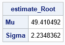
The estimates are the same as those obtained by optimizing the 2-D log-likelihood function. However, it is generally easier and more reliable to solve for a 1-D root. Of course, you do have to specify a search interval for σ, but you can use the MoM estimates to help with that task.

Summary

In SAS, you can use PROC UNIVARIATE (or PROC SEVERITY) to obtain maximum likelihood estimates. Although PROC UNIVARIATE and PROC SEVERITY support about 20 common distributions, it can be useful to know how to solve these problems in SAS IML in case you need to fit a distribution that is not natively supported in SAS. This article shows three methods to obtain parameter estimates for a univariate distribution. Each method is demonstrated by using the Gumbel distribution. The methods are:

The method of moments (MoM) is an old technique that uses sample moments to estimate the parameters. The MoM estimates are also useful as an initial guess for an MLE optimization.
A traditional maximum likelihood estimation optimizes the log-likelihood function. You can use the MoM estimates as an initial guess. This article uses the NLPQN (Quasi-Newton method) to find the parameters that maximize the log-likelihood function.
You can use calculus to obtain a system of equations for the MLEs. For simple distributions (eg, Normal and Lognormal), you can solve these equations to obtain the parameter estimates. For other distributions, the equations decouple, and you can reduce the optimization to a root-finding method. This article shows how to use the FROOT function in IML to estimate a parameter by solving for a 1-D root. For the Gumbel distribution, it is helpful to know about the sum-of-exponentials trick, which you can use to improve the numerical stability of the computation.

Blogs