Many common probability distributions contain terms that increase or decrease quickly, such as the exponential function and factorials. The numerical evaluation of these quantities can result in numerical overflow (or underflow). This is why we often work on the logarithmic scale: on the log-scale, the numerical computations for equations such as the log-likelihood function are more stable.

This article demonstrates a different trick that is useful for computing a sum of exponential terms. I have seen it called the sum-of-exponentials trick. When used on the log scale, some researchers call it the log-sum-of-exponentials trick.

Motivation: The Gumbel distribution and sum of exponentials

Recently, I needed to work with the Gumbel distribution. The Gumbel distribution presents numerical challenges because it is doubly exponential. For example, the density function is given by the doubly exponential formula f(x) = (1/σ) exp(-(z + exp(-z))), where z = (x - μ)/σ and where μ is a location parameter and σ is a scale parameter,

If you collect a random sample of data {x1, x2, ..., xn}, you can fit a Gumbel distribution to the data by using the loglikelihood function for the Gumbel distribution. As I will show in a subsequent article, fitting the Gumbel distribution involves an expression that looks like this:
     $R = \frac{\sum_{i=1}^{n}x_i \exp(-x_i/\sigma)} {\sum_{i=1}^{n}\exp(-x_i/\sigma)}.$

Notice that the numerator and denominator both contain a sum of exponential terms. If you don't handle those sums carefully, they could experience numerical overflow or underflow. Specifically, if the denominator underflows (that is, evaluates to 0), then you will get a "division by zero" error, and the ratio cannot be computed. Fortunately, there is a numerical trick that is useful for computing with a sum of exponentials: Shift the argument of the exponential function to obtain a more stable computation.

Why does the EXP function cause problems?

Before we look at sums, let's look at a single call to the EXP function.

The exponential function, EXP(x), increases really fast as x increases in the positive direction. It also decreases very fast as x decreases in the negative direction. In standard double-precision (64-bit) floating-point computations, the largest representable number is 1.7977E308. However, the logarithm of that huge number is only 709.783, which means that the numerical argument of the EXP function cannot exceed 709.783. In addition to the numbers that tell you when the EXP function will overflow, there are analogous numbers related to underflow.

These numbers are so important that SAS software provides a function that returns them. In SAS, you can use the CONSTANT function to find the value of constants that are important in numerical computations. The following DATA step creates these numbers:

data ExpConstants;
Small = constant('small');
Logsmall = constant('logsmall');
Logbig = constant('logbig');
Big = constant('big');
run;
 
proc print noobs; run;

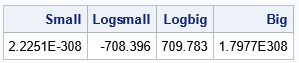
The constants labeled Small and Logsmall are related to underflow of the EXP function. Mathematically, the quantity exp(x) > 0 for all real values of x. But the smallest positive representable number is about 2.2251E-308. The log of that number is -708.396. Consequently, the EXP function will return 0 for any x < -708.396. This can cause problems, for example, if you are dividing by exp(x). If x is too negative, you could get a division-by-zero error.

The following DATA step demonstrates overflow and underflow for the EXP function. The EXP function underflows (that is, returns 0) for x < 709.783:

%macro OverUnder;
   if y=0 then Computation='Underflow';
   else if y=. then Computation='Overflow ';
   else Computation='Okay     ';
%mend;
 
data ExpUnderOverFlow(drop=Logbig Logsmall);
Logsmall = constant('logsmall');
Logbig = constant('logbig');
x = floor(Logsmall); y = exp(x); %OverUnder; output;
x = Logsmall;        y = exp(x); %OverUnder; output;
x = Logbig;          y = exp(x); %OverUnder; output;
x = ceil(Logbig);    y = exp(x); %OverUnder; output;
label y = "y=EXP(x)";
run;
 
proc print noobs label; run;

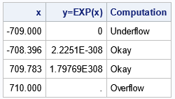
The table shows four values of x and EXP(x). If Logsmall ≤ x ≤ Logbig, then EXP(x) returns a valid value. Otherwise, the function underflows (returns 0) or overflows (returns missing).

Shifting the argument of the EXP function

A common mathematical trick is to multiply an expression by 1 in a clever way so that parts of the expression simplify. Let c be any real number. Then exp(c)*exp(-c) = 1, so we can rewrite any expression exp(t) as
     $\exp(t) = \exp(c) \exp(t - c)$

How does this help? Well, you can use c to stabilize the computation. For example, if t = -800, then exp(t) underflows. However, if you choose c appropriately, you can represent exp(t) as a product of two terms that can each be computed. For example, if c= -300, then exp(t) = exp(c)*exp(t-c) = exp(-300)*exp(-400). Note that exp(-300) and exp(-400) can both be computed, even though the product cannot be.

The next section demonstrates this trick for a sum of exponential terms.

Shifting the argument of a sum of exponentials

Let's return to sums. Let $S= \sum_{i=1}^{n}\exp(t_i)$ be an exponential sum for any set of numbers $\{t_1, t_2, \ldots, t_n\}$. By the reasoning in the previous section, you can represent each term of the sum as $\exp(t_i) = \exp(c) \exp(t_i - c)$, so the sum becomes
     $S = \exp(c) \sum_{i=1}^{n}\exp(t_i - c)$
where we have pulled exp(c) outside the summation. If you choose c appropriately, S is the product of exp(c) and a sum that can be computed.

Let's see the trick in action for the term in the denominator of the ratio, R. The following small data set contains numbers that are close to 5. The program reads the data into an IML vector and computes the sum of exponentials with and without the trick.

/* define sample data */
data MyData;
input x @@;
datalines;
4.68 4.80 5.01 4.97 5.05 4.99
;
 
proc iml;
use MyData; read all var {'x'}; close;
 
/* when sigma is not too small, the computations are straightforward */
sigma = 0.5;
t = -x / sigma;        /* this expression is used in some statistical computations */
print x t;
Denom = sum(exp(t));   /* no trick used here; just sum the exponents */
print sigma Denom;
 
/* the sum-of-exponent trick enables you to robustly compute sum(exp(t)) */
c = min(t);         /* or mean or max ... */
A = exp(c);         /* this term might over- or underflow */
B = sum(exp(t-c));  /* hopefully, this term is stable */
print A B (A*B)[L='A*B'];

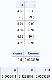
The first table shows the values of x and of t, which is a simple linear transformation of x. When the parameter sigma is not too small, the values of t are all within the domain of the EXP function. In this case, there are no numerical problems. You can compute the quantity Σ_i exp(t_i) in a straightforward manner, as shown in the second output table.

The last output table shows the result of applying the sum-of-exponentials trick. You can use any value of c, but I chose c = min(t) so that the quantity (t - c) is always positive. Regardless, the trick enables you to convert the sum of exponents into a product. One factor is exp(c) and the other is a modified sum. The last table shows these values as well as the product. For this example, the product has the same value as the straightforward sum of exponents. In the next section, we apply the sum-of-exponentials trick to the ratio of sums, R.

The sum-of-exponentials trick for ratios

The previous section showed that the sum of the exponential term is (mathematically) the same whether or not you shift the exponential terms by a constant. The sum-of-exponentials trick is most useful when computing a ratio that involves the sum of exponents. A ratio that comes up in the MLE estimation of the Gumbel distribution is the following:
     $R = \frac{\sum_{i=1}^{n}x_i \exp(-x_i/\sigma)} {\sum_{i=1}^{n}\exp(-x_i/\sigma)}.$

Let t_i = -x_i/σ. If you apply the sum-of-exponentials trick to both the numerator and denominator (using the same value of c), you get the following identity:
     $R = \frac{\exp(c) \sum_{i=1}^{n}x_i \exp(t-c)} {\exp(c) \sum_{i=1}^{n} \exp(t-c)} = \frac{\sum_{i=1}^{n}x_i \exp(t-c)} {\sum_{i=1}^{n} \exp(t-c)}$

Notice that the exp(c) terms cancel! This means that we can stabilize the sum-of-exponentials even if the expression exp(c) will overflow or underflow!

Let's see how this works by revisiting the previous example in PROC IML.

/* decrease sigma so that t is not in the domain of the EXP function.
   Bad things happen if we aren't careful! */
sigma = 0.005;
t = -x / sigma;
print x t;
Denom = sum(exp(t));    /* underflow */
print sigma Denom;
 
/* Use the sum-of-exponentials trick for ratios */
c = min(t);
A = exp(c);         /* might over- or underflow */
Denom = sum(exp(t-c));  /* stable */
Numer = sum(x#exp(t-c));  /* stable */
R = Numer / Denom;
print A Numer Denom R;

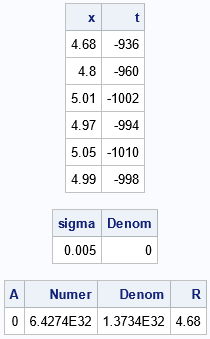
When σ is small enough, the quantity -x[i]/sigma is a large negative number, which means that EXP will underflow. You can see that the straightforward computation of the denominator equals 0, which means that we cannot compute the ratio. However, if we use the trick, we can set c = -1010 and factor exp(c) out of the terms in the sum. Because exp(c) appears in both the numerator and denominator, we never have to compute that number! Consequently, we can compute the ratio.

Summary

This article shows the sum-of-exponentials trick. For any constant, c, the expression exp(t) = exp(c)*exp(t-c). This enables you to express the computation as a product. In practice, you choose c so that exp(t-c) will not overflow or underflow. This often means that exp(c) is a "bad term" that will over- or underflow. However, if the computation is part of a ratio, the "bad terms" cancel, enabling you to compute the ratio in a numerically stable way.

A follow-up article applies the trick to the maximum likelihood estimate for the Gumbel distribution.