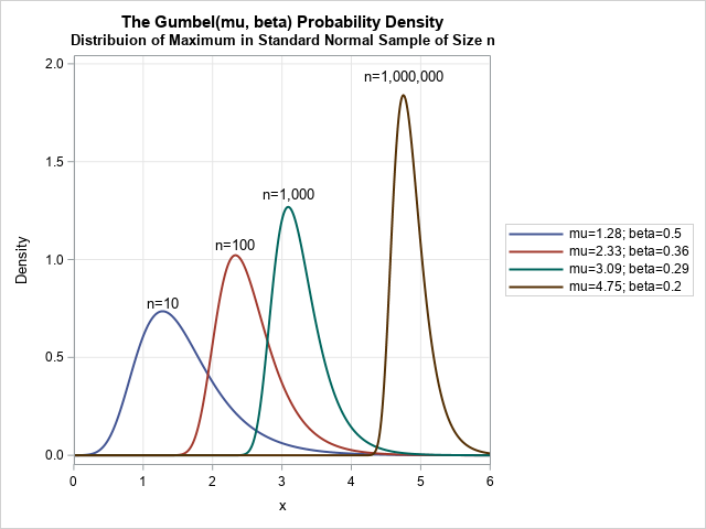
SAS supports more than 25 common probability distributions for the PDF, CDF, QUANTILE, and RAND functions. Of course, there are infinitely many distributions, so not every possible distribution is supported. If you need a less-common distribution, I've shown how to extend the functionality of Base SAS (by using PROC FCMP) or the SAS/IML language by defining your own functions. This article shows how to implement the Gumbel distribution in SAS. The density functions for four parameter values of the Gumbel distribution are shown to the right. As I recently discussed, the Gumbel distribution is used to model the maximum (or minimum) in a sample of size n.

Essential functions for the Gumbel Distribution

If you are going to work with a probability distribution, you need at least four essential functions: The CDF (cumulative distribution), the PDF (probability density), the QUANTILE function (inverse CDF), and a way to generate random values from the distribution. Because the RAND function in SAS supports the Gumbel distribution, you only need to define the CDF, PDF, and QUANTILE functions.

These functions are trivial to implement for the Gumbel distribution because each has an explicit formula. The following list defines each function. To match the documentation for the RAND function and PROC UNIVARIATE (which both support the Gumbel distribution), μ is used for the location parameter and σ is used for the scale parameter:

• CDF: F(x; μ, σ) = exp(-exp(-z)), where z = (x - μ) / σ
• PDF: f(x; μ, σ) = exp(-z-exp(-z)) / σ, where z = (x - μ) / σ
• QUANTILE: F^-1(p; μ, σ) = μ - σ log(-log(p)), where LOG is the natural logarithm.

The RAND function in Base SAS and the RANDGEN function in SAS/IML support generating random Gumbel variates. Alternatively, you could generate u ~ U(0,1) and then use the QUANTILE formula to transform u into a random Gumbel variate.

Using these definitions, you can implement the functions as inline functions, or you can create a function call, such as in the following SAS/IML program:

proc iml;
start CDFGumbel(x, mu, sigma);
   z = (x-mu)/sigma;
   return exp(-exp(-z));                   * CDF of Gumbel distribution;
finish;
 
start PDFGumbel(x, mu, sigma);
   z = (x-mu)/sigma;
   return exp(-z-exp(-z)) / sigma; 
finish;
 
start QuantileGumbel(p, mu, sigma);
   return mu - sigma # log(-log(p));
finish;
 
/* Example: Call the PDFGumbel function */
mu = 3.09;                       /* params for max value of a sample of size */
sigma = 0.286;                   /*       n=1000 from the std normal distrib */
x = do(2, 5, 0.025);
PDF = PDFGumbel(x, mu, sigma);
title "Gumbel PDF";
call series(x, PDF) grid={x y};

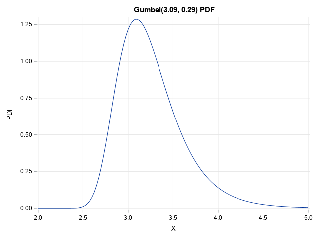
The graph shows the density for the Gumbel(3.09, 0.286) distribution, which models the distribution of the maximum value in a sample of size n=1000 drawn from the standard normal distribution. You can see that the maximum value is typically between 2.5 and 4.5, which values near 3 being the most likely.

Plot a family of Gumbel curves

I recently discussed the best way to draw a family of curves in SAS by using PROC SGPLOT. The following DATA step defines the PDF and CDF for a family of Gumbel distributions. You can use this data set to display several curves that indicate how the distribution changes for various values of the parameters.

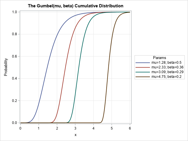
data Gumbel;
array n[4] _temporary_     (10   100  1000 1E6);   /* sample size */
array mu[4] _temporary_    (1.28 2.33 3.09 4.75);  /* Gumbel location parameter */
array beta [4] _temporary_ (0.5  0.36 0.29 0.2);   /* Gumbel scale parameter */
do i = 1 to dim(beta);                       /* parameters in the outer loop */
   m = mu[i]; b = beta[i];
   Params = catt("mu=", m, "; beta=", b);    /* concatenate parameters */
   do x = 0 to 6 by 0.01;
      z = (x-m)/b;
      CDF = exp( -exp(-z));                  /* CDF for Gumbel */
      PDF = exp(-z - exp(-z)) / b;           /* PDF for Gumbel */
      output;
   end;
end;
drop z;
run;
 
/* Use ODS GRAPHICS / ATTRPRIORITY=NONE 
   if you want to force the line attributes to vary in the HTML destination. */
title "The Gumbel(mu, beta) Cumulative Distribution";
proc sgplot data=Gumbel;
   label cdf="Probability";
   series x=x y=cdf / group=Params lineattrs=(thickness=2);
   keylegend / position=right;
   xaxis grid;  yaxis grid;
run;
 
title "The Gumbel(mu, beta) Probability Density";
proc sgplot data=Gumbel;
   label pdf="Density";
   series x=x y=pdf / group=Params lineattrs=(thickness=2);
   keylegend / position=right;
   xaxis grid offsetmin=0 offsetmax=0;  yaxis grid;
run;
 
title "The Gumbel(mu, beta) Quantile Function";
proc sgplot data=Gumbel;
   label cdf="Probability";
   series x=cdf y=x / group=Params lineattrs=(thickness=2);
   keylegend / position=right sortorder=reverseauto;
   xaxis grid;  yaxis grid;
run;

The graph for the CDF is shown. A graph for the PDF is shown at the top of this article. I augmented the PDF curve with labels that show the sample size for which the Gumbel distribution is associated. The leftmost curve is the distribution of the maximum in a sample of size n=10; the rightmost curve is for a sample of size one million.

Random values and fitting parameters to data

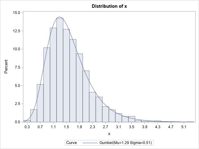
For completeness, I will mention that you can use the RAND function to generate random values and use PROC UNIVARIATE to fit Gumbel parameters to data. For example, the following DATA step generates 5,000 random variates from Gumbel(1.28, 0.5). The call to PROC UNIVARIATE fits a Gumbel model to the data. The estimates for (μ, σ) are (1.29, 0.51).

data GumbelRand;
call streaminit(12345);
mu = 1.28;
beta = 0.5;
do i = 1 to 5000;
   x = rand("Gumbel", mu, beta);
   output;
end;
keep x;
run;
 
proc univariate data=GumbelRand;
   histogram x / Gumbel;
run;

In summary, although the PDF, CDF, and QUANTILE functions in SAS do not support the Gumbel distribution, it is trivial to implement these functions. This article visualizes the PDF and CDF of the Gumbel distributions for several parameter values. It also shows how to simulate random values from a Gumbel distribution and how to fit the Gumbel model to data.