Order variables by using a loading plot

The article "Order two-dimensional vectors by using angles" shows how to re-order a set of 2-D vectors by their angles. Because angles are on a circle, which has no beginning and no end, you must specify which vector will appear first in the list. The previous article finds the largest gap between angles and uses it to determine the first vector.

A statistical application of this technique is to reorder the variables in a correlation analysis by using a loading plot or a similar visualization. The loading plot is typically based on a principal component analysis (PCA), so an equivalent statement is that this technique reorders the variables by using a PCA.

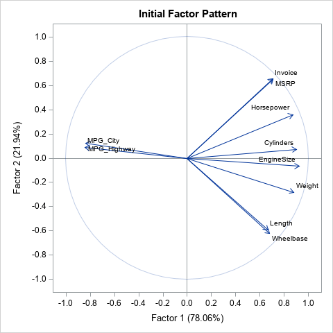
In SAS, the PRINCOMP and FACTOR procedures can automatically create a loading plot, as shown to the right. If the first two principal components capture most of the variation in the data, then variables (vectors) that have a small angle between are highly correlated. Similarly, variables that have a large angle between them tend to be uncorrelated or negatively correlated.

This article shows how to ensure that the loading plot and the correlation matrix use the same ordering of the variables. Vectors that have a small angle between them are adjacent to each other in the rows and columns of the correlation matrix. For this example, the desired ordering of the variables is Wheelbase, Length, Weight, ..., MPG_Highway, MPG_City.

Example data and a loading plot

The graph to the right is created from the Sashelp.Cars data by using the following SAS statements:

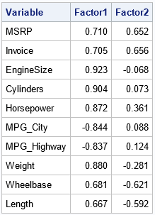
%let DSOut = Vectors;          /* data set for coordinates of vectors */ 
%let DSName = Sashelp.Cars;    /* input data set */
%let varNames = _NUMERIC_;     /* which variables to analyze? */
proc factor data=&DSName method=principal N=2 /* N= specifies number of factors */
     plots=(initloadings(vector));
   var &varNames;
   ods output InitPatternPlot=&DSOut;         /* store the vector coordinates */
run;
 
/* the data in the InitPatternPlot contains the set of 2-D vectors and variable names */
proc print data=&DSOut noobs;
   var Variable Factor1 Factor2;
   format _numeric_ 6.3;
run;

The &DSOut data set contains the coordinates and labels for the vectors shown in the loading plot. (The observant reader will notice that the MPG_City vector is "south" of the MPG_Highway vector. To avoid overplotting, the labels on the loading plot are displaced from their exact positions.) The next section reads the coordinates into IML vectors and applies the sorting algorithm from the previous article.

Order vectors by their angles

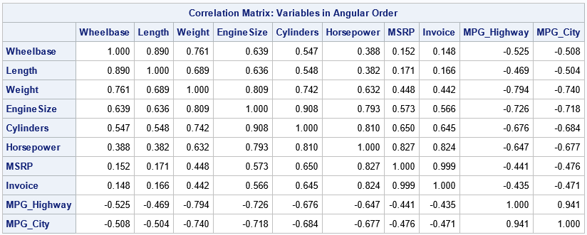
The Appendix lists a SAS IML function (Sort2DVecByAngle) that was developed in a previous article. The following IML program loads the Sort2DVecByAngle function and loads the data for the vectors. The call to Sort2DVecByAngle returns a permutation that sorts the vectors. You can use this permutation to sort the variable names. If you use this ordering to perform a correlation analysis, the rows and columns of the correlation matrix are in the same order as the loading plot, which is Wheelbase, Length, ..., MPG_Highway, MPG_City. This is shown in the following program:

proc iml;
LOAD module=Sort2DVecByAngle;    /* assume this function was previously stored (or define it here) */
 
/* read in vectors */
use &DSOut;
   read all var {Factor1 Factor2} into V;
   read all var "Variable" into vNames;
close;
 
order = Sort2DVecByAngle(V);   /* call the function that orders the vectors */
varNames = vNames[order];      /* reorder the variable names */
 
/* use the sort order to visualize the correlation matrix */
/* read the original variables and compute correlation. */
use &DSName;
   read all var varNames into Y;
close;
corr = corr(Y);
print corr[c=varNames r=varNames F=6.3 L="Correlation Matrix: Variables in Angular Order"];

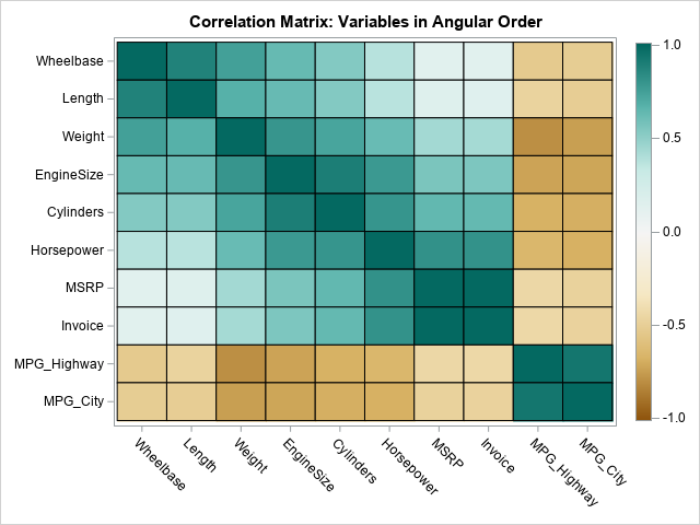
If you want to visualize the correlation matrix by using a heat map, you can use the HEATMAPCONT subroutine in IML, as follows:

colors = palette("BrBg", 7);      /* get the Brown-to-Bluegreen color ramp */
call HeatmapCont(corr) xvalues=varNames yvalues=varNames 
            colorramp=colors range={-1.01 1.01} 
            title="Correlation Matrix: Variables in Angular Order";

The rows and columns of the heat map display the variables in the same order as the loading plot. Variables that are highly correlated with each other (such as Wheelbase and Length) appear next to each other in the heat map.

I want to point out that this ordering method, which is conceptually easy, gives essentially the same result as the more complicated "single-link cluster algorithm" for this example. The ordering algorithm is much easier to implement than the single-link cluster algorithm.

Export the variable order

If you want to use the new variable order outside of IML, you can write the new order into a string. You can then use the SYMPUTX call to create a SAS macro variable and use the macro variable on the VAR statement of procedures such as PROC CORR. The following example uses the Vec_To_Str function to convert the vector of variable names into a string:

/* Concatenate a character vector into a single string of blank-separated values.
   If you want exactly one space between elements, use this function.
   If you don't mind extra spaces, you can use ROWCAT(ROWVEC(s)+" ");
   See https://blogs.sas.com/content/iml/2024/11/13/vector-to-string-2.html
*/
start vec_to_str(s);
   c1 = cat(rowvec(s), ' ');   /* add blank at end */
   c2 = compbl(rowcat(c1));    /* concatenate values and compress blanks */
   return trim(c2);            /* remove the extra blank at the end of the string */
finish;
 
names = vec_to_str(varNames);         /* concatenate variable names into a string */
call symputx("sortedVarList", names); /* write string to macro variable */
QUIT;
 
/* Example: use the sortedVarList macro variable to perform correlation analysis outside PROC IML */
proc corr data=&DSName noprob nosimple nomiss; 
   var &sortedVarList;
run;

The output is not shown, but it is equivalent to the table of correlations shown earlier.

Summary

The loading plot is a convenient way to visualize the correlation of vectors by using a principal component analysis. If the first two principal components explain most of the variance, the angles between vectors in the loading plot are a good way to visualize the correlation between variables. It makes sense, therefore, to want to construct a correlation matrix or heat map whose rows and columns use the same variable ordering as the loading plot. This article shows how to use a SAS IML module (see the Appendix) to perform the computation. You can copy the new variable order into a macro variable to use it in other procedures.

Appendix: The Sort2DVecByAngle function in SAS IML

The following SAS IML module sorts a set of 2-D vectors according to their angles. The function is explained in a previous article. The input argument is an (n x 2) matrix, V. The rows of V are 2-D vectors in the plane. The function returns a permutation of the vectors 1:n that sorts the rows in order of the vector angles. The largest angular gap determines the first and last vector.

proc iml;
/* V is an (n x 2) matrix where the rows of V are 2-D vectors in the plane. 
   Return a permutation that sorts the rows so that the vectors are sorted
   in order of angles. The first and last vector have the largest gap between them.
*/
start Sort2DVecByAngle(V);
   /* compute angles each vector makes with X axis 
      See https://blogs.sas.com/content/iml/2015/06/10/polar-angle-curve.html */
   pi = constant('pi');
   n = nrow(V);
   theta = atan2(V[,2],V[,1]); /* angle in range (-pi, pi] */
   ndx = loc(theta<0); /* eliminate jump discontinuity at theta=pi by using [0, 2*pi) */
   if ncol(ndx)>0 then 
      theta[ndx] = theta[ndx] + 2*pi;
 
   /* sort angles */
   call sortndx(sortIdx, theta);   /* sort index */
   theta = theta[sortIdx];
 
   /* compute difference between consecutive angles (including last minus first) */
   gap = dif(theta//(2*pi+theta[1]), 1,1); /* discard first obs (.) in difference vector */
   maxIdx = gap[<:>];      /* find the largest gap */
 
   /* if maxIdx=n, vectors are in correct sequence; otherwise, reorder */
   if maxIdx < n then do;
      firstIdx = maxIdx+1;
      gIdx = firstIdx:n || (1:(firstIdx-1));
      SortIdx  = SortIdx[gIdx];
   end;
   return SortIdx;
finish;
STORE module=Sort2DVecByAngle;
QUIT;

Blogs