Confidence limits for counts in a multinomial distribution

A recent article discussed Pareto charts and how to create them in SAS. A Pareto chart is used in quality control to identify the most likely reasons that a manufacturing process produces defective items. Suppose there are k different reasons why a process can fail, and you intend to randomly select N defective items to examine. The number of defective items for each reason can be modeled by using a multinomial distribution.

A variation of the Pareto chart (Wilkinson, TAS, 2006) uses confidence intervals for multinomial counts to enhance the information on the chart. This article supplies the necessary background for how to estimate confidence intervals for multinomial counts. A subsequent article shows how to construct Wilkinson's Pareto chart in SAS.

The multinomial distribution

Suppose a categorical variable, X, can take on k different values. A statistical model of the variable is to assume that X can be modeled by a multinomial distribution. A multinomial distribution assumes that the probability of the i_th value is p_i, where Σ_i p_i = 1.

In a sample of size N, there will be N₁ items of the first type, N₂ items of the second type, and so forth, where Σ_i N_i = N. The k-tuple of counts (N₁, N₂, ..., N_k) is a single observation from the multinomial distribution.

The expected value of N_i is N*p_i, but in an actual sample the count could be higher or lower than that value. Confidence intervals enable you to answer the question, "what is the likely range of each count?"

A previous article describes how to construct simultaneous confidence intervals for the proportions. But the Wilkinson variation of the Pareto chart uses marginal confidence limits, which are different. Marginal confidence limits can be easily generated by running a simulation of the multinomial distribution and using percentiles of the results. In SAS, the easiest way to simulate from the multinomial distribution is to use the RandMultinomial function in SAS IML.

Simulating multinomial frequencies

Suppose a quality engineer samples 40 defective items. She finds that there are six causes for the defective items. In the sample, N₁=17 items are defective because of the first cause, N₂=10 are defective because of the second cause, and the remaining causes are responsible for 5, 3, 3, and 2 counts, respectively. The best estimate of the unknown probabilities is obtained by dividing the counts by N=40. Thus, the empirical probabilities are p = {0.425, 0.25, 0.125, 0.075, 0.075, 0.05}.

The following call to PROC IML specifies these parameters and generates five random samples. Each sample is a random draw from the multinomial distribution.

/* CI for marginal probability parameters in a multinomial distribution */
proc iml;
/* observed frequencies */
freq = {17, 10, 5, 3, 3, 2};
N = sum(freq);      /* sample size */
p = freq / N;
 
/* 5 random samples of size N from Multinom(p) */
call randseed(123);
X5 = randmultinomial(5, N, p);
print X5[c=('C1':'C6') r=('S1':'S5')];

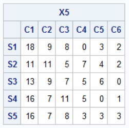
Each row shows the count in a random sample. The i_th column shows the counts for the i_th defective cause across all five samples. In this small simulation, the counts for the first cause range from 11-18, the counts for the second cause range from 7-11, and so forth. Because the probabilities for the 4th-6th causes are relatively small, some samples did not contain any items for those causes.

The small output gives us the intuition behind confidence intervals. We'd like to know ranges that cover the counts for 95% of the samples. You can do this by generating a large number of samples and calculating percentiles.

Confidence intervals for the multinomial counts

The previous output shows the range of counts for each variable for five random samples. Now imagine generating many more random samples from the same multinomial distribution. If you compute the 2.5th and 97.5th percentiles for each column, you obtain a simulation-based estimate of a 95% confidence interval for each column's values. The following IML statements perform these calculations for a simulation that uses 10,000 random draws.

/* Use simulation to estimate (1-alpha)*100% confidence intervals 
   for counts for each category.
   - N = sample size
   - p = parameter vector for Multinomial(N, p) distribution
   - B is the number of Monte Carlo simulations
   - alpha = significance level (default 0.05) ==> 95% CL   
*/
start MultinomialCL(B, N, p, alpha=0.05);
   X = RandMultinomial(B, N, p); /* generate B random samples */
   /* Find the (alpha / 2) and (1 - alpha / 2) percentiles.
      For alpha = 0.05, this estimates the 2.5th and 97.5th percentiles. */
   w = (alpha/2) // (1-alpha/2);
   call qntl(CL, X, w);       /* QNTL computes the quantiles of each column */
   return( CL );
finish;
 
/* call function and print the results in a table */
limits = MultinomialCL(10000, N, p);
Category = 'C1':'C6';
print limits[r={'Lower95' 'Upper95'} c=Category L="Marginal Limits (N=40)"];

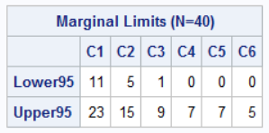
The table shows 95% confidence limits for the counts from a multinomial sample of size N=40 that has a vector of probability parameters p. For the most probable category (C1), you can expect the count to be between 11 and 23 for 95% of samples. For the least probable category (C6), you can expect the count to be between 0 and 5.

Although the table provides all relevant information, I like to graph the confidence intervals as bars in a chart that graphs the observed frequency and confidence intervals versus the categories, as follows:

/* graph the empirical frequencies and the marginal CLs */
Lower95 = limits[1,];
Upper95 = limits[2,];
create MultinomialLimits var {'Category' 'Freq' 'Lower95' 'Upper95'};
   append;
close;
QUIT;
 
title "95% Confidence Limits for Frequencies";
proc sgplot data=MultinomialLimits noautolegend;
   highlow x=Category low=Lower95 high=Upper95 / 
           type=bar barwidth=0.8;* primary=true;
   scatter x=Category y=Freq;
   yaxis offsetmin=0 grid;
   xaxis type=discrete discreteorder=data;
run;

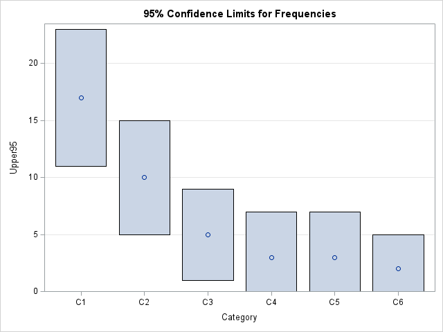
The graph enables you to see at a glance the ranges of counts for a sample of size N from the multinomial(N, p) distribution.

Summary

The statistics of small random samples can be highly variable. This article looks at the counts in a multinomial distribution. By running a simple simulation study, you can construct 95% confidence intervals for the counts. This is helpful for quality engineers who need to know whether an increase or decrease in an observed count is associated with a change in the manufacturing process or is merely random variation. These confidence intervals are used in constructing Wilkinson's variation of the Pareto chart, which I will construct in a future article.

Blogs