A categorical response variable can take on k different values. If you have a random sample from a multinomial response, the sample proportions estimate the proportion of each category in the population. This article describes how to construct simultaneous confidence intervals for the proportions as described in the 1997 paper "A SAS macro for constructing simultaneous confidence intervals for multinomial proportions" by Warren May and William Johnson (Computer Methods and Programs in Biomedicine, p. 153–162).

Estimates of multinomial proportions

In their paper, May and Johnson present data for a random sample of 220 psychiatric patients who were categorized as either neurotic, depressed, schizophrenic or having a personality disorder. The observed counts for each diagnosis are as follows:

data Psych;
input Category $21. Count;
datalines;
Neurotic              91
Depressed             49
Schizophrenic         37
Personality disorder  43
;

If you divide each count by the total sample size, you obtain estimates for the proportion of patients in each category in the population. However, the researchers wanted to compute simultaneous confidence intervals (CIs) for the parameters. The next section shows several methods for computing the CIs.

Methods of computing simultaneous confidence intervals

May and Johnson discussed six different methods for computing simultaneous CIs. In the following, 1–α is the desired overall coverage probability for the confidence intervals, χ²(α, k-1) is the upper 1–α quantile of the χ² distribution with k-1 degrees of freedom, and π₁, π₂, ..., π_k are the true population parameters. The methods and the references for the methods are:

1. Quesenberry and Hurst (1964): Find the parameters π_i that satisfy
   N (p_i - π_i)² ≤ χ²(α, k-1) π_i(1-π_i).
2. Goodman (1965): Use a Bonferroni adjustment and find the parameters that satisfy
   N (p_i - π_i)² ≤ χ²(α/k, 1) π_i(1-π_i).
3. Binomial estimate of variance: For a binomial variable, you can bound the variance by using π_i(1-π_i) ≤ 1/4. You can construct a conservative CI for the multinomial proportions by finding the parameters that satisfy
   N (p_i - π_i)² ≤ χ²(α, 1) (1/4).
   
4. Fitzpatrick and Scott (1987): You can ignore the magnitude of the proportion when bounding the variance to obtain confidence intervals that are all the same length, regardless of the number of categories (k) or the observed proportions. The formula is
   N (p_i - π_i)² ≤ c²(1/4)
   where the value c²= χ²(α/2, 1) for α ≤ 0.016 and where c²= (8/9)χ²(α/3, 1) for 0.016 < α ≤ 0.15.
5. Q and H with sample variance: You can replace the unknown population variances by the sample variances in the Quesenberry and Hurst formula to get
   N (p_i - π_i)² ≤ χ²(α, k-1) p_i(1-p_i).
6. Goodman with sample variance: You can replace the unknown population variances by the sample variances in the Goodman Bonferroni-adjusted formula to get
   N (p_i - π_i)² ≤ χ²(α/k, 1) p_i(1-p_i).

In a separate paper, May and Johnson used simulations to test the coverage probability of each of these formulas. They conclude that the simple Bonferroni-adjusted formula of Goodman (second in the list) "performs well in most practical situations when the number of categories is greater than 2 and each cell count is greater than 5, provided the number of categories is not too large." In comparison, the methods that use the sample variance (fourth and fifth in the list) are "poor." The remaining methods "perform reasonably well with respect to coverage probability but are often too wide."

A nice feature of the Q&H and Goodman methods (first and second on the list) is that they procduce unsymmetric intervals that are always within the interval [0,1]. In contrast, the other intervals are symmetric and might not be a subset of [0,1] for extremely small or large sample proportions.

Computing CIs for multinomial proportions

You can download SAS/IML functions that are based on May and Johnson's paper and macro. The original macro used SAS/IML version 6, so I have updated the program to use a more modern syntax. I wrote two "driver" functions:

• CALL MultCIPrint(Category, Count, alpha, Method) prints a table that shows the point estimates and simultaneous CIs for the counts, where the arguments to the function are as follows:
  • Category is a vector of the k categories.
  • Count is a vector of the k counts.
  • alpha is the significance level for the (1-alpha) CIs. The default value is alpha=0.05.
  • Method is a number 1, 2, ..., 6 that indicates the method for computing confidence intervals. The previous list shows the method number for each of the six methods. The default value is Method=2, which is the Goodman (1965) Bonferroni-adjusted method.
• MultCI(Count, alpha, Method) is a function that returns a three-column matrix that contains the point estimates, lower limit, and upper limit for the CIs. The arguments are the same as above, except that the function does not use the Category vector.

Let's demonstrate how to call these functions on the psychiatric data. The following program assumes that the function definitions are stored in a file called CONINTS.sas; you might have to specify a complete path. The PROC IML step loads the definitions and the data and calls the MultCIPrint routine and requests the Goodman method (method=2):

%include "conint.sas";   /* specify full path name to file */
proc iml;
load module=(MultCI MultCIPrint);
use Psych; read all var {"Category" "Count"}; close;
 
alpha = 0.05;
call MultCIPrint(Category, Count, alpha, 2); /* Goodman = 2 */

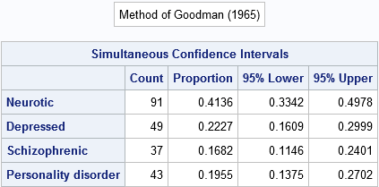
The table shows the point estimates and 95% simultaneous CIs for this sample of size 220. If the intervals are wider than you expect, remember the goal: for 95% of random samples of size 220 this method should produce a four-dimensional region that contains all four parameters.

You can visualize the width of these intervals by creating a graph. The easiest way is to write the results to a SAS data set. To get the results in a matrix, call the MultCI function, as follows:

CI = MultCI(Count, alpha, 2);  /*or simply CI = MultCI(Count) */
/* write estimates and CIs to data set */
Estimate = CI[,1];  Lower = CI[,2];  Upper = CI[,3];
create CIs var {"Category" "Estimate" "Lower" "Upper"};
append;
close;
quit;
 
ods graphics / width=600px height=240px;
title 'Simultaneous Confidence Intervals for Multinomial Proportions';
title2 'Method of Goodman (1965)';
proc sgplot data=CIs;
  scatter x=Estimate y=Category / xerrorlower=Lower xerrorupper=upper
          markerattrs=(Size=12  symbol=DiamondFilled)
          errorbarattrs=GraphOutlines(thickness=2);
  xaxis grid label="Proportion" values=(0.1 to 0.5 by 0.05);
  yaxis reverse display=(nolabel);
run;

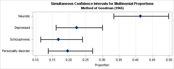
The graph shows intervals that are likely to enclose all four parameters simultaneously. The neurotic proportion in the population is probably in the range [0.33, 0.50] and at the same time the depressed proportion is in the range [0.16, 0.30] and so forth. Notice that the CIs are not symmetric about the point estimates; this is most noticeable for the smaller proportions such as the schizophrenic category.

Because the cell counts are all relatively large and because the number of categories is relatively small, Goodman's CIs should perform well.

I will mention that it you use the Fitzpatrick and Scott method (method=4), you will get different CIs from those reported in May and Johnson's paper. The original May and Johnson macro contained a bug that was corrected in a later version (personal communication with Warren May, 25FEB2016).

Conclusions

This article presents a set of SAS/IML functions that implement six methods for computing simultaneous confidence intervals for multinomial proportions. The functions are updated versions of the macro %CONINT, which was presented in May and Johnson (1987). You can use the MultCIPrint function to print a table of statistics and CIs, or you can use the MultCI function to retrieve that information into a SAS/IML matrix.