I've been working on a project that uses quasi-Monte Carlo (QMC) techniques to estimate probabilities for multivariate normal (MVN) distributions on finite or infinite rectangular regions. The goal is to enable SAS users to compute these probabilities accurately and efficiently.
My implementation is based on a numerical technique called the Genz transformation (A. Genz, 1992; Genz and Bretz, 2009, pp. 49-50). It leverages the geometric fact that the Cholesky factor of a correlation matrix provides a transformation that maps uncorrelated MVN variables to correlated MVN variables. I previously wrote about using the Cholesky transformation to correlate variables, and Genz's method is a clever and useful application of this linear algebraic technique. The technique goes back to multivariate statistical methods developed by Mahalanobis in the 1930s.
This article discusses the Genz transformation method and shows how to compute and visualize the integrand for a bivariate normal distribution. This low-dimensional example demonstrates the main ideas that are used in higher dimensions.
The computation of MVN probabilities
The goal is to estimate the probability that a random multivariate normal vector falls inside a specific rectangular region:
\( P( L_1 < X_1 < U_1, L_2 < X_2 < U_2, \dots, L_d < X_d < U_d ) \)
where (X1, X2, ..., Xd) ~ MVN(0, Σ), and Σ is the covariance matrix. The lower and upper limits are defined by the vectors L = (L1, L2, ..., Ld) and U = (U1, U2, ..., Ud).
We'll adopt the convention that each Li is less than Ui and we'll allow
elements of L to represent negative infinity and elements of U to represent positive infinity.
In SAS, you can use the special missing value .M to represent minus infinity and .I to represent positive infinity.
The probability is formally computed by evaluating a multidimensional integral:
\(
\int_{L_1}^{U_1} \int_{L_2}^{U_2} \cdots \int_{L_d}^{U_d} \phi(x; \Sigma)\, dx
\)
where φ(x; Σ) is the MVN density function.
Does that integral look scary to you? Because it looks scary to me! In numerical analysis, there are not many good ways to solve high-dimensional integrals. For low to moderate dimensions, you can use ordinary Monte Carlo simulations to estimate this probability. There are two common Monte Carlo techniques:
- The Region method (a.k.a., "naive Monte Carlo"): Generate B random variates Xi ~ MVN(0, Σ) and calculate the proportion of the Xi inside the rectangular region defined by the limits. For completeness, the Appendix shows a traditional Monte Carlo implementation of the region method.
- The Average Function method: Evaluate a certain function for B random variates in the domain of the function. Compute the average of the values. I am intentionally leaving "the function" and "the domain" unspecified for now. As we will soon see, Genz transforms the domain of the problem, and the function that gets evaluated is somewhat complicated.
For the Average Function method, you can generate quasi-random variates and perform a quasi-Monte Carlo analysis. A quasi-Monte Carlo estimate has a smaller standard error than a naive Monte Carlo estimate that uses the same number of points.
Unfortunately, QMC methods are limited to finite regions because
quasi-random sequences are generated inside the unit hypercube.
Genz solved this issue by transforming the general MVN region into an equivalent integration problem strictly on the unit hypercube. Because the innermost integral can be evaluated analytically, a d-dimensional probability reduces to an integral over the (d-1)-dimensional hypercube:
\( \int_{(0,1)^{d-1}} g(w) \, dw \)
where the integrand, g, depends on the covariance matrix and the limits of integration.
You can use QMC techniques to efficiently estimate the integral with high accuracy.
You generate N quasi-random points in the (d-1)-dimensional hypercube, evaluate the function g at each point,
and take the average, as follows:
\( p \approx \frac{1}{N} \sum_{i=1}^N g(w_i) \)
Of course, there is no such thing as a free lunch, so the Genz integration function, g, is more complicated than the standard MVN density function. But Genz's paper was seminal because it shows how to evaluate the integral by using linear transformations and the inverse CDF transformation.
An overview of the Genz transformation
Genz's method consists of three main steps:
- The Cholesky transformation: Transform the problem from correlated variables into independent standard normal variables. This transformation has been known since the 1930s.
- Conditional probability: When integrating the i_th variable, you must condition the bounds on the exact values drawn for the previous (i-1) dimensions. This step uses conditional probability to update the lower and upper limits of integration for each variable.
- The inverse CDF Transformation: You can use the inverse CDF transformation to map these updated bounds into the unit hypercube.
A 2-D Implementation in SAS IML
Although Genz's algorithm works in arbitrary dimensions, let's use it to integrate the MVN probability in 2-D. SAS already has functions for evaluating the bivariate normal probability, so we can use those functions to check whether we implemented Genz's method correctly.
Assume L and U are row vectors. The following SAS IML program defines two helper functions to handle infinite bounds for the CDF("Normal") function. The main function is called GenzIntegrand_2D.
As input parameters, it takes two-element vectors L and U and a 2x2 correlation matrix, R.
It also takes a vector of values, w, in the interval (0,1).
There are several ways you can use that input argument. I will use it to visualize the
function by passing in a grid of values on the interval (0,1). However, if you want to average the
function to estimate the 2-D MVN probability, you would send in a set of quasi-random numbers in (0,1) and average the output.
The Genz transformation "integrates out" the innermost variable in the problem. As a result, the Genz integrand is a function of one fewer variables than the original problem. For a 2-D probability, the Genz integrand is a 1-D function. For a 3-D probability, the integrand is a function of two variables, and so forth.
The following SAS IML program begins with three helper functions. The main function is GenzIntegrand_2D. The comments in the function indicate the three main steps for transforming the bivariate normal probability into a 1-D function that can be integrated.
proc iml; /* Helper functions: Extend the CDF function so that / 0 if x = -Infinity cdf(x) = { cdf(x) if x is finite \ 1 if x = +Infinity */ start cdf_at_lower(L); if L=. then return( 0 ); /* = cdf("Normal", -Infinity) */ return( cdf("Normal", L) ); finish; start cdf_at_upper(U); if U=. then return( 1 ); /* = cdf("Normal", +Infinity) */ return( cdf("Normal", U) ); finish; /* The Title2_from function sets the TITLE2 statement dynamically at runtime. See https://blogs.sas.com/content/iml/2015/01/14/global-statements-loops.html The string looks like "rho=0.5; P(. < X1 < 2 & -2 < X2 < 1)" */ %macro char(x); choose(&x=., ".", char(&x)) %mend; start Title2_from(L, U, rho); rhoStr = cats("rho=",char(rho),";"); range1 = cats(%char(L[1]),"< X1 <",%char(U[1])); range2 = cats(%char(L[2]),"< X2 <",%char(U[2])); parmStr = catx(" ", rhoStr, "P(", range1, "&", range2, ")"); call execute("title2 '" + parmStr + "';" ); finish; /* The Genz method transforms a vector of independent standard normal variables Y ~ MVN(0, I) into the observed correlated variables X~MVN(0, R) by using the Cholesky factor, C. In 2-D, relates X to Y via the linear equations X1 = C11*Y1 X2 = C21*Y1 + C22*Y2 */ start GenzIntegrand_2D(w, L, U, R); /* The ROOT function returns an upper triangular matrix. Transpose to get lower triangular */ C = t(root(R)); /* First dimension (outer integral) */ v1 = 0; /* (un)conditional mean of X1 */ c11 = C[1,1]; /* Standardize limits and calculate probability mass M1 */ alpha = cdf_at_lower( (L[1]-v1)/c11 ); beta = cdf_at_upper( (U[1]-v1)/c11 ); M1 = beta - alpha; /* 1-D marginal probability */ /* The inverse CDF maps each w in (0,1) to normal variable y1. Note: y1 is a vector in (-Infinity, Infinity) */ y1 = quantile("Normal", alpha + w * M1); /* Second dimension (inner integral) */ c21 = C[2,1]; c22 = C[2,2]; /* Conditional mean depends on the y1 from the previous step. Subtract the conditional mean and standardize limits for inner integral. */ v2 = c21 * y1; alpha = cdf_at_lower( (L[2]-v2)/c22 ); beta = cdf_at_upper( (U[2]-v2)/c22 ); M2 = beta - alpha; /* Final integrand: M1 is a scalar, M2 is a vector, so g is a vector. */ g = M1 * M2; return (g); finish; /* Visualize the 1-D integrand for the following 2-D problem */ rho = 0.5; R = (1 || rho) // (rho || 1 ); L = {.M -1}; U = { 1 2}; /* Evaluate and plot the Genz integrand, which is defined on the open interval (0,1) */ w = {1E-4, 5E-4, 0.001, 0.005} // T(do(0.01, 0.99, 0.01)) // {0.995, 0.999, 0.9995, 0.999}; g = GenzIntegrand_2D(w, L, U, R); title "Genz Integrand for 2-D MVN"; call Title2_from(L, U, rho); xLabel = "w (Uniform QMC Coordinate)"; yLabel = "g(w) = Probability Mass"; call series(w, g) grid={X Y} label=xLabel other=cat("yaxis grid min=0 label='",yLabel,"';"); |
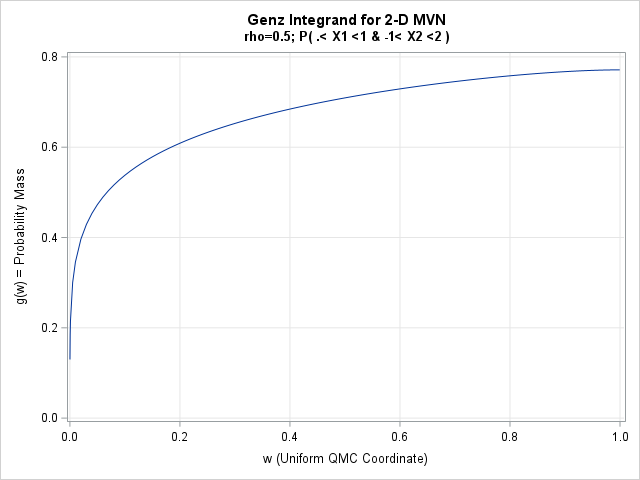
The resulting curve represents the integrand for the transformed integration problem. To find the true MVN probability in the region, you integrate the function over the interval (0,1). You can estimate the integral by evaluating the function on a 1-D QMC sequence, then taking the average. Visually, the probability is the average height of this smooth positive function.
Since this is a bivariate problem, you can use SAS to find that the true probability is about 0.677. Notice that this value is the average height of the function on (0, 1).
The Genz integrand for uncorrelated variables
If the correlation matrix for a MVN distribution is the identity, the problem decomposes into a product of univariate marginal probabilities. The Genz integrand for this situation is a straight line. The height of the line is the probability value. To see this fact in action, let's use a very small value of rho so that the function will be almost a horizontal line.
/* If you use a tiny value for rho, the integrand approaches a constant function. When rho=0 exactly, the integrand is the product of the two marginal probabilities. The function becomes a constant. */ rho = 0.01; /* prob = 0.6882697 for this value of rho */ R = (1 || rho) // (rho || 1 ); g = GenzIntegrand_2D(w, L, U, R); call Title2_from(L, U, rho); call series(w, g) grid={X Y} label=xLabel other=cat("yaxis grid min=0 max=0.75 label='",yLabel,"';"); |
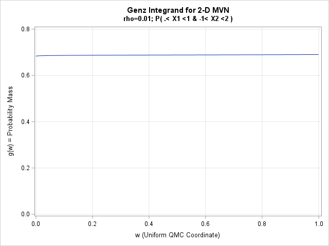
As expected, the Genz integrand is very close to a horizontal line. The height of the curve is very close to 0.688, which is the probability value for this problem. The curve becomes a horizontal line for rho=0.
The Genz integrand for small probabilities
One of the problems with a Monte Carlo simulation that uses the "Region method" is that the method requires many random variates to get an accurate estimate. For example, if you set rho=-0.5, the bivariate normal probability P( X1 < -1 & -3 < X2 < -2 ) = 0.000145. If you use the Monte Carlo "Region method" to estimate the probability, you would expect only 145 points per million to be inside the region of interest. Most variates are "wasted" because they are outside of the region. In contrast, the Genz transformation of this problem does not waste any evaluations. The Genz integrand is very short, but every value in (0,1) contributes to the average value of g on (0, 1). This is shown in the following program:
/* What does the integrand look like if we use a negative rho and specify a region in which the probability is small? */ rho = -0.5; R = (1 || rho) // (rho || 1 ); L = {.M -3}; U = {-1 -2}; g = GenzIntegrand_2D(w, L, U, R); call Title2_from(L, U, rho); call series(w, g) grid={X Y} label=xLabel other=cat("yaxis grid min=0 label='",yLabel,"';"); |
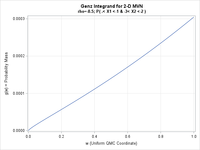
As expected, the integrand is very small. The maximum value of the function on (0, 1) is approximately 0.0003. The function is approximately linear and g(0) ≈ 0, so a quick back-of-the-envelope calculation of the probability is 0.00015, which is pretty doggone close to the true value! You could estimate the probability by using only a few thousand quasi-random points in (0,1), which is a huge savings over the millions of points that are required for a naive Monte Carlo estimate.
Summary
This article presents a general computational framework for estimating a probability for a rectangular region of a multivariate normal distribution. Three bivariate examples are given: a problem where the variables are moderately correlated, a problem where the variables are almost independent, and an example where the probability is very small. For each case, I visualize the Genz integrand, which is a 1-D function. By integrating the Genz integrand, you obtain the desired probability. You can use quasi-Monte Carlo integration, which amounts to evaluating the integrand many times and taking the average.
The algorithm generalizes to higher dimensions. For a d-dimensional MVN distribution, the Genz integrand is a function of d-1 variables that each have (0, 1) as a domain. Thus, the problem reduces to estimating the integral of a function on the unit hypercube, which can be computed efficiently by using quasi-Monte Carlo methods.
Appendix: The traditional Monte Carlo estimate
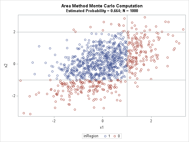
As mentioned in the article, the Genz transformation is more efficient than the traditional Monte Carlo estimates. For example, the following PROC IML program simulates N=1000 points from the bivariate normal distribution with ρ = 0.5 that is shown in the first graph. For this run, using 1000 data points results in an estimated probability of 0.664. The true probability of 0.677, so the estimate is not bad. However, the standard error of the Monte Carlo method is proportional to 1/sqrt(N), whereas the Genz transformation and quasi-random integration has a much smaller standard error proportional to 1/N.
proc iml; rho = 0.5; R = (1 || rho) // (rho || 1 ); L = {.M -1}; U = { 1 2}; /* Visualize the Monte Carlo estimate P(X1< 1 && -1 < X2 < 2) */ N = 1000; call randseed(123, 1); X = randnormal(N, {0 0}, R); hit = (X[,1] < U[1]) && (L[2] < X[,2] && X[,2] < U[2]); p_est = mean(hit); print p_est; result = X||hit; create MCViz from result[c={'x1' 'x2' 'inRegion'}]; append from result; close; quit; title "Area Method Monte Carlo Computation"; title2 "Estimated Probability = 0.664; N = 1000"; proc sgplot data=MCViz; scatter x=x1 y=x2 / group=inRegion; refline 1 / axis=x; refline -1 2 / axis=y; run; |