This article shows how to use SAS to compute the probabilities for two correlated normal variables. Specifically, this article shows how to compute the probabilities for rectangular regions in the plane. A second article discusses the computation over infinite regions such as quadrants.

If (X,Y) are random variables that are jointly distributed according to a probability density function, f(x,y), then the probability that (X,Y) are inside any planar region, R, is given by the following double integral:
      $\mathbf{P}((X,Y) \in R) = \iint\limits_{(x,y) \in R} f(x,y) \,dx \,dy$
A rectangular region in the plane can be represented as the product of two intervals: R = (a,b) x (c,d). In this case, the probability is
      $\mathbf{P}(a < X < b, \, c < Y < d) = \int_c^d \int_a^b f(x,y) \,dx \,dy$

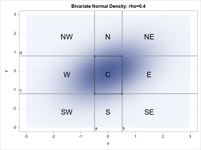
For example, the graph to the right overlays a "tic-tac-toe" grid on a contour plot of the standard bivariate normal density with correlation ρ=0.4. The central rectangle (marked "C") is the region (-0.5, 0.5) x (-1.2, 0.8). This article shows that the bivariate normal probability for that region is about 0.27. That is, the probability is 0.27 that a random variate from the specified distribution is observed in the "C" region.

The phrase "standard bivariate normal distribution with correlation ρ" is quite long to write. I will use the notation BVN(0, ρ) to represent the standard bivariate normal distribution with correlation ρ.

Notation for the standard bivariate normal distribution

In this article, we restrict to the standard bivariate normal density function (PDF) with correlation ρ, which is given by
$\phi(x,y; \rho)=\frac{1}{2 \pi \sqrt{1-\rho^2}} \exp \left(-\left( x^2-2\rho x y+y^2 \right) / (2 (1-\rho^2)) \right)$
The corresponding cumulative distribution function, represented by a capital "phi", Φ, is the integral of the PDF over the quadrant (-∞,b) x (-∞,d):
$\Phi(x,y; \rho) = \mathbf{P}(X < x, Y < y) = \int_{-\infty}^y \int_{-\infty}^x \phi(u,v; \rho) \,du \,dv$

If those integrals look scary, fear not! SAS provides the PROBBNRM function, which enables you to compute Φ(x,y; ρ) for any finite values (x,y). No integration is required to evaluate Φ. A previous article discusses the PROBBNRM function and shows a graph of Φ(x,y; 0).

It turns out that the PROBBNRM function is all you need to compute the BVN probability for any rectangular region. Before showing the bivariate computation, the next section quickly reviews the computation of probability for the standard univariate normal distribution.

Probability for the standard univariate normal distribution

The computation of probability for the standard univariate normal distribution is well known, so it is a perfect place to start. Recall that the SAS function CDF("Normal", x) computes the left-tailed probability
$\mathbf{P}(X < x) = \int_{-\infty}^x \phi_1(u) \,du$
where X ~ N(0,1) is a random variable that is standard normal, and φ₁ is the corresponding univariate PDF.

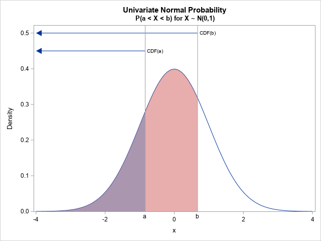
Notice that the CDF is defined as a left-tail probability. It only has one argument, which is the upper limit of the integral. So, how do you compute the probability that X is in some interval, such as (a,b)? You evaluate the CDF at the right side of the interval (CDF(b)) and then subtract the CDF at the left side of the interval. Therefore, the probability P(a < X < b) = CDF(b) - CDF(a).

This is illustrated by the graph at the right. The quantity CDF(b) is the sum of the pink and purple areas under the curve. The purple area is CDF(a). Thus, the pink area represents the probability that X is in (a,b). The pink area is evaluated as CDF(b) - CDF(a).

The bivariate case

The univariate case reminds us that the CDF function evaluates the left-tail probability P(X < x), which is equivalent to an integration of the density function over the domain (-∞, x). The bivariate case is similar, except now the CDF is a function of two variables. The analogue of a "left-tail" probability is a "southwest quadrant" probability.

The PROBBNRM function in SAS evaluates the standard bivariate normal density over the "southwest quadrant" that is determined by the argument. For example, in the graph at the top of this article, the region marked "SW" is the region below and to the left of the point (a,c) = (-0.5, -1.2). You can compute the probability over that region by using the following call to the PROBBNRM function, which evaluates the PROBBNRM function at (a,c) when ρ=0.4:

/* show examples of using the PROBBNRM function */
data ProbSW;
rho = 0.4;
a = -0.5; b =  0.5;  /* cut points in X direction */
c = -1.2; d =  0.8;  /* cut points in Y direction */
SWProb = probbnrm(a, c, rho);
run;
 
proc print data=ProbSW noobs; 
   var rho a c SWProb;
run;

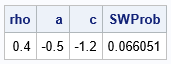
The output shows that the probability is 0.066 that a random variate from BVN(0, ρ) will be observed in the "SW" region.

The probability over a finite rectangular region

You can use the PROBBNRM function to evaluate the probability that a random variate is in any of the nine regions in the graph. Eight of the regions are infinite, so let's start by discussing how to evaluate the probability for the central (finite) rectangular region marked "C" in the plot, which is the region (a,b) x (c,d) in the graph. To evaluate the probability, proceed as follows:

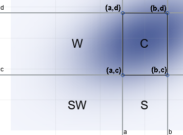
1. Evaluate the bivariate CDF at (b,d). This gives the probability for the quadrant that is the union of the four areas C, W, S, and SW.
2. Let's try to get rid of the excess probability. Evaluate the bivariate CDF at (a,d). This gives the probability over the union of the two areas W and SW. If we subtract this probability from the prior calculation, the result is the probability over the regions C and S. We are getting closer to our goal!
3. We need to get rid of the probability associated with the region S. Evaluate the bivariate CDF at (b,c). This gives the probability over the union of the two areas S and SW. If we subtract this probability from the prior calculation, we obtain the probability over the regions C minus the probability over the region SW.
4. We have subtracted too much, so we need to add back the probability associated with the region SW. To do this, evaluate the bivariate CDF at (a,c). This gives the probability over SW. Add that value to the previous result.

Thus, you can obtain the BVN probability in the rectangle (a,b) x (c,d) by performing the following computations:

data ProbRect;
rho = 0.4;
a = -0.5; b =  0.5;  /* cut points in X direction */
c = -1.2; d =  0.8;  /* cut points in Y direction */
bdProb = probbnrm(b, d, rho);   /* upper right corner */
adProb = probbnrm(a, d, rho);   /* upper left corner  */
bcProb = probbnrm(b, c, rho);   /* lower right corner */
acProb = probbnrm(a, c, rho);   /* lower left corner  */
rectProb = bdProb - adProb - bcProb + acProb;
run;
 
proc print data=ProbRect noobs; 
   var rho a b c d rectProb;
run;

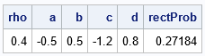
The probability is 0.27 that a random variate from BVN(0, 0.4) is observed in the rectangle.

Notice the similarity to the univariate case. A one-dimensional interval has two endpoints. You obtain the probability on a one-dimensional interval by evaluating the CDF at the right endpoint and subtracting the CDF at the left endpoint. In two dimensions, a rectangular region has four corners. You obtain the probability on a rectangle by evaluating the CDF at the four corners and performing a sequence of additions and subtractions.

Probability as a function of the correlation

The previous section shows how to compute a bivariate normal probability on a rectangle for the correlation ρ=0.4. It is straightforward to modify the program to compute the probability for any BVN(0, ρ) distribution. In fact, you can compute the probability for a sequence of ρ values by using a loop. You can then visualize how the probability in the rectangle changes as a function of the correlation:

/* compute probability in rectangle for a sequence of rho values */
data ProbRho;
a = -0.5; b =  0.5;  /* cut points in X direction */
c = -1.2; d =  0.8;  /* cut points in Y direction */
do rho = -0.95 to 0.95 by 0.01;
   bdProb = probbnrm(b, d, rho);   /* upper right corner */
   adProb = probbnrm(a, d, rho);   /* upper left corner  */
   bcProb = probbnrm(b, c, rho);   /* lower right corner */
   acProb = probbnrm(a, c, rho);   /* lower left corner  */
   rectProb = bdProb - adProb - bcProb + acProb;
   output;
end;
keep a b c d rho rectProb;
run;
 
title "Probability in a Rectangular Region";
title2 "(-0.5, 0.5) x (-1.2, 0.8)";
proc sgplot data=ProbRho;
   series x=rho y=rectProb;
   xaxis grid;
   yaxis grid;
   label rho="Correlation (rho)" rectProb="P(a<X<b,c<Y<d; rho)";
run;

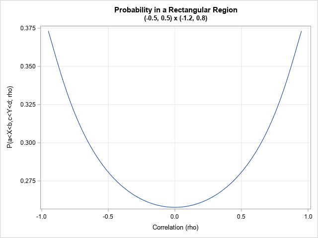
For this region, the graph is symmetric, which means that the probability is the same for BVN(0,ρ) and BVN(0,-ρ). The probability for this region is the smallest when ρ=0 and increases as ρ approaches ±1.

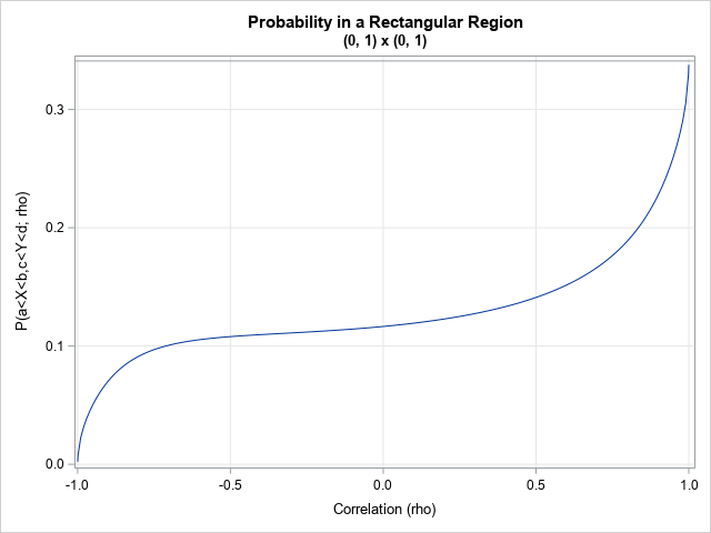
If you choose a different rectangular region, you will get a different graph. For example, change the region to B = (0,1) x (0,1) and rerun the program. You will get a graph that looks like the following. The region B is in the "northeast" quadrant relative to the point (0,0), so for a BVN distribution that has a very negative correlation, almost none of the probability in the region B. On the other hand, for a BVN distribution that is almost perfectly correlated, the probability is concentrated near the line identity line y=x. You can show that the probability in B is 0.341 for the limiting distribution that has ρ=1. That number equals CDF(1) – CDF(0) for the univariate normal CDF.

Summary

In SAS, you can use the PROBBNRM function to evaluate the bivariate normal CDF for any correlation -1 < ρ < 1. This article shows how you can use the bivariate normal distribution function to compute the probability associated with two types of planar regions. If (X,Y) are standard bivariate normal random variables with correlation ρ, then

• The function call PROBBNRM(x,y,rho) returns the probability P(X < x, Y < y). This is the infinite "southwest quadrant" region that is defined by the point (x,y).
• To evaluate the probability in the rectangle (a,b) x (c,d), use the expression
  probbnrm(b,d,rho) - probbnrm(a,d,rho) - probbnrm(b,c,rho) + probbnrm(a,c,rho)

The graph at the top of this article shows nine regions, each having a different shape. This article shows how to find the probability for the SW and C regions. A separate article shows how to use the bivariate CDF to compute probabilities for the other regions.