A previous article discussed how to compute probabilities for the bivariate standard normal distribution. The standard bivariate normal distribution with correlation ρ is denoted BVN(0,ρ). For any point (x,y), you can use the PROBBNRM function in SAS to compute the probability that the random variables (X,Y) ~ BVN(0,ρ) is observed in the "southwest quadrant": P(X < x, Y < y). Thus, PROBBNRM evaluates the two-dimensional CDF for the BVN(0,ρ) distribution.

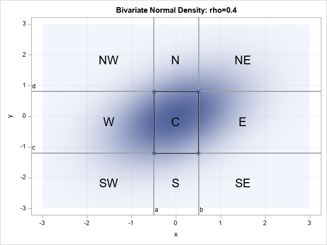
For example, the graph at the right overlays four reference lines on a contour plot of the density of the BVN(0, ρ) distribution where ρ=0.4. In SAS, a call to PROBBNRM(-0.5, -1.2, 0.4) computes the probability in the region marked "SW". The previous article also showed how to compute the probability in the rectangular region marked "C" by evaluating the PROBBNRM function at the four corners of the rectangle and using the expression
probbnrm(b,d,rho) - probbnrm(a,d,rho) - probbnrm(b,c,rho) + probbnrm(a,c,rho)

The other regions do not have four corners, so you might wonder how to generalize this idea to the other regions in the figure. The infinite regions have either one or two points that define the region. Nevertheless, this article shows that you can use the PROBBNRM function to evaluate the probability of any region in the figure by thinking of the other "corners" as being points at infinity.

Extending the PROBBNRM function to handle infinity

To evaluate the probability on the infinite regions, we need to use some mathematical properties of the standard bivariate normal CDF. For brevity, denote the bivariate CDF as Φ and the CDF of the univariate normal distribution as Φ₁. Then the following statements are true (Kotz, Balakrishnan, Johnson (2000), Continuous Multivariate Distributions, Vol 1, 2nd Ed, p 264-265):

• The limit as y → ∞ of Φ(x,y; ρ) is Φ₁(x) for all -1 ≤ ρ ≤ 1. In an abuse of notation, we can write Φ(x,∞; ρ) = Φ₁(x).
• Similarly, by symmetry, Φ(∞, y; ρ) = Φ₁(y) for all ρ.

You can use these facts to extend the PROBBNRM function so that it can return the probability associate with a left half plane, which is Φ(x,∞; ρ). Similarly, you can compute the probability in the lower half plane, which is Φ(∞, y; ρ). In SAS, I will use the special missing value .P to denote positive infinity. It will also be convenient to use the special missing value .M to represent negative infinity.

The previous article used the SAS DATA step to evaluate the PROBBNRM function. In this article, I use the SAS IML language because a future article uses these computations to perform maximum likelihood estimation. The following statements define a SAS IML function that extends the two-dimensional CDF to support infinity as an upper limit. The program tests the function by computing the probability associated with the left half plane {(x,y) | x < 0.5} and the lower half plane {(x,y) | y < 0.8}. Of course, the area of the complementary right- and upper half planes are simple to compute:

proc iml;
/* Extend the bivariate CDF, which is PROBBNRM(a,b, rho) to support an 
   upper limit of infinity (.P) for either argument:
   Pr(u,.P; rho) = Phi(u) = cdf("Normal", u) is probability over left half plane
   Pr(.P,v; rho) = Phi(v) = cdf("Normal", v) is probability over lower half plane
*/
start CDFBN(u,v,rho);
   if missing(u) & missing(v) then 
      return 1;
   if missing(u) then 
      return cdf("Normal", v);
   if missing(v) then 
      return cdf("Normal", u);
   return probbnrm(u, v, rho);
finish;
 
rho = 0.4;
x0 = 0.5; y0 = 0.8;
 
/* probability for half planes */
probLeft  = CDFBN(x0, .P, rho); /* left half plane {(x,y) | x < x0} */
probRight = 1 - probLeft;       /* right half plane */
probLower = CDFBN(.P, y0, rho); /* lower half plane {(x,y) | y < y0} */
probUpper = 1 - probLower;      /* upper half plane */
print probLeft probRight probLower probUpper;

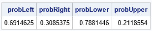
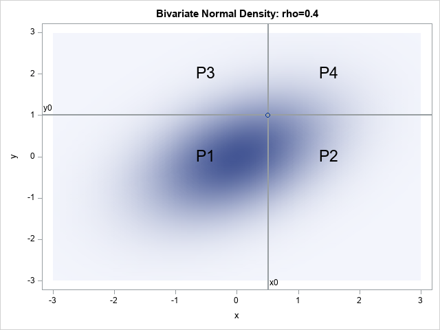
The output shows the BVN probability that is associated with the half planes. The probability for the left half plane {(x,y) | x < 0.5} is 0.69. In the graph at the right, this is the probability in the regions marked P1 and P3. The probability for the lower half plane {(x,y) | y < 0.8} is 0.79. In the graph, this is the probability in the regions marked P1 and P2.

You can use the CDFBN function to obtain the probability for any quadrant. For example, the point (x0, y0) defines the four regions shown in the graph to the right. The following statements compute the probability for the BVN(0, 0.4) distribution in each region:

/* use half planes to compute quadrants */
P1 = CDFBN(x0, y0, rho);        /* probability SW from (x0,y0) */
P2 = CDFBN(.P, y0, rho) - P1;   /* probability SE from (x0,y0) */
P3 = CDFBN(x0,.P, rho) - P1;    /* probability NW from (x0,y0) */
P4 = 1 - (P1 + P2 + P3);        /* probability NE from (x0,y0) */
print P1 P2 P3 P4;
QUIT;

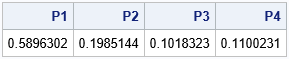
You should interpret the output as follows. If you generate a random variate from the BVN(0, 0.4) distribution, there is a 59% chance that the observation will be in the lower left region (P1), a 20% chance the observation will be in the lower right region, a 10% chance it will be in the upper left region, and an 11% chance it will be in the upper right region.

The probability in any finite or infinite rectangular region

You can create a function, ProbBVN(a,b,c,d, rho), that can compute the BVN(0, ρ) probability for any rectangular region of the form (a,b) x (c,d). The function can support infinite intervals such as (-∞, b) and (-∞, d) by specifying a=.M or c=.M. Similarly, the function can support infinite intervals such as (a, ∞) and (c, ∞) by specifying b=.P or c=.P. By considering all the combinations of ways that the (a,b,c,d) arguments can be finite or missing, the ProbBVN function can support 16 different region shapes, including quadrants, half planes, strips, half strips, and finite rectangles.

You can download the SAS IML function definitions from GitHub. The following SAS IML program shows how to call the function to compute the areas of the nine regions in the graph at the top of this article:

proc iml;
load module=(CDFBN ProbBVN);   /* the CDFBN and ProbBVN functions must be stored by using the STORE statement */
 
rho = 0.4;
a = -0.5; b =  0.5;
c = -1.2; d =  0.8;
Prob = j(nrow(desc), 1, .);
Prob[1] = ProbBVN(.M,  a, .M,  c, rho);   /* SW */
Prob[2] = ProbBVN( a,  b, .M,  c, rho);   /* S  */
Prob[3] = ProbBVN( b, .P, .M,  c, rho);   /* SE */
Prob[4] = ProbBVN(.M,  a,  c,  d, rho);   /* W  */
Prob[5] = ProbBVN( a,  b,  c,  d, rho);   /* C  */
Prob[6] = ProbBVN( b, .P,  c,  d, rho);   /* E  */
Prob[7] = ProbBVN(.M,  a,  d, .P, rho);   /* NW */
Prob[8] = ProbBVN( a,  b,  d, .P, rho);   /* N  */
Prob[9] = ProbBVN( b, .P,  d, .P, rho);   /* NE */

If you print the probabilities and the intervals for each region, you obtain the following table:

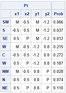
Most of the probability is in the "C" rectangle and the "W" half strip. The quadrants "SE" and "NW" contain the least probability. Notice that the sum of the probabilities is 1, as it must be.

By considering sums, you can also get the probability in the following regions:

• Left, right, lower, and upper half planes. For example, the sum NW + W + SW is the probability in the half plane {(x,y) | x < a}.
• Vertical and horizontal strips. For example, the sum S + C + N is the probability in the vertical strip {(x,y) | a < x < b}.
• The entire plane. However, we know in advance that the probability over the entire plane is 1.

Thus, the ProbBVN function supports computing the probability in 16 different region shapes. The nine shapes shown in the graph above are the most common shapes for statistical applications.

Summary

SAS provides the PROBBNRM function, which evaluates the bivariate standard normal CDF for any finite point (x,y). This gives you the probability that a random variate is in the "southwest" quadrant {(u,v) | u < x, v < y}. You can use the PROBBNRM function to compute probabilities a finite rectangle and for a few other regions. This article shows that you can extend the 2-D CDF function to also compute the probability in half planes. The extended functionality enables you to define a new function, ProbBVN(a,b,c,d, rho), which computes the bivariate probability in the region (a,b) x (c,d). In addition to finite values, you can use a=.M, b=.P, c=.M, and d=.P to specify infinite regions, where the special SAS missing values .M and .P are used to represent -∞ and +∞, respectively.

You can download the SAS programs that were used to generate the graphs and tables in this article from GitHub.