Why are some dispersion statistics re-scaled?

In statistics, the normal (Gaussian) distribution serves as a reference for many statistical quantities. For example, a normal distribution has excess kurtosis equal to zero, and other distributions are classified as leptokurtic (heavier-than-normal tails) or platykurtic (lighter-than-normal tails) in comparison.

Similarly, the standard deviation of a normal distribution (σ) is often used as a reference for other dispersion statistics. Specifically, when you use a robust measure of spread such as the interquartile range (IQR) or the median of absolute deviations (MAD), those measures are often adjusted so that they are consistent with the standard deviation for normally distributed data.

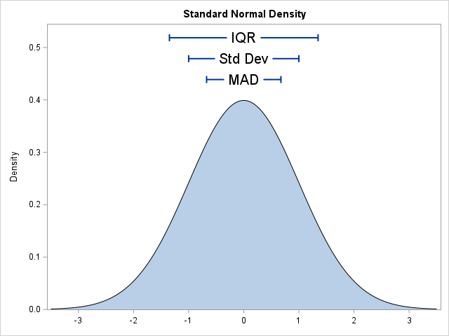
The graph to the right shows the standard deviation, IQR, and MAD for a standard normal distribution. You can see that the MAD is smaller than the standard deviation whereas the IQR is larger. It is useful to re-scale the IQR and MAD quantities so that they equal the standard deviation for the normal distribution. For example, the MAD is too short, so the quantity 1.4826*MAD is often used as a robust estimate of scale for contaminated normal data. The constant 1.4826 "adjusts" or "re-scales" the MAD statistic so that it estimates the standard deviation (σ) in a set of normally distributed data.

In a similar way, the IQR is "too large," so you will often see the quantity 0.7413*IQR, which is another robust estimate for σ.

Where do these constants come from? In these two cases, they can be derived theoretically, as shown in the Appendix. But this article shows that you can also use a Monte Carlo simulation to obtain those values. A simulation enables you to empirically solve for the scale factors that convert the MAD and IQR into consistent estimators of σ. You can use the simulation to adjust any dispersion statistic so that it estimates the standard deviation for normally distributed data.

It turns out that you can also use the sample RANGE to form a consistent estimator of the standard deviation. However, the expected value of the range depends on the sample size, so the scale factor is not constant but is a function, called d₂(n). SAS/QC provides a function to compute D2, or you can use SAS/IML to evaluate the function by solving an integral.

Robust Measures in PROC UNIVARIATE

The ROBUSTSCALE option in the PROC UNIVARIATE statement computes several robust measures of scale. It not only calculates the raw MAD and IQR but also includes a multiplicative scaling factor that scales them to estimate σ. The scaling factor for each robust statistic is shown in the PROC UNIVARIATE documentation. Let's see how these factors work. The following SAS DATA step simulates 100 observations from a standard normal distribution. The standard deviation of the population is 1.0. The call to PROC UNIVARIATE requests robust measures of scale:

/* generate a random sample from N(0,1) */
%let N = 100;
data SimNormal1;
call streaminit(12345);
do i = 1 to &n;
    x = rand("Normal");
    output;
end;
keep x;
run;
 
/* The ROBUSTSCALE option on the PROC UNIVARIATE statement computes robust measures of scale */
proc univariate data=SimNormal1 robustscale;
    var x;
    ods select BasicMeasures RobustScale;
run;

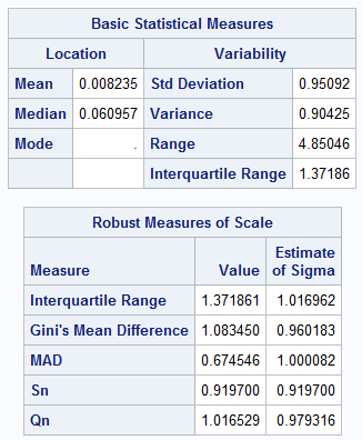
The first table shows some descriptive statistics, including the sample standard deviation (0.951), which is the usual estimate for σ. The second table shows some robust measures of scale, including the IQR and MAD statistics. The first column displays the robust statistics, the second column (labeled "Estimate of Sigma") shows the value after multiplying by an appropriate constant. This is the "re-scaled" statistic. It is an estimate of σ for the special case when the data are normally distributed. Notice that all entries in the second column are somewhat close to 1 because these data are, in fact, normally distributed from a population for which σ = 1. For the MAD statistic, the second column equals 1.4826 · MAD; for the IQR statistic, the second column equals 0.7413 · IQR. The next section shows how to create a Monte Carlo simulation to estimate these constants.

A Monte Carlo simulation to approximate the sampling distribution of MAD and IQR

We want to find constants for which the expected value of the MAD and IQR statistics are consistent with the standard deviation for normal data. In other words, for normally distributes data, we want to find constants for which:

k_IQR · E[IQR] = σ, which implies that k_IQR = σ / E[IQR].
k_MAD · E[MAD] = σ, which implies that k_MAD = σ / E[MAD].

The following Monte Carlo simulation generates 10,000 random samples from N(0,1) and computes the MAD and IQR statistics for each sample. The statistics are written to a SAS data set named RS.

/* Monte-Carlo simulation: Generate 10,000 random samples from N(0,1) */
%let N = 100;
%let numSamples = 10000;
data SimNormal;
call streaminit(12345);
do sampleID = 1 to &numSamples;
   do i = 1 to &n;
      x = rand("Normal");
      output;
   end;
end;
keep sampleID x;
run;
 
/* approximate the sampling distribution of MAD and IQR */
ods exclude all;
proc univariate data=SimNormal robustscale;
    by sampleID;
    var x;
    ods output RobustScale=RS;
run;
ods exclude none;

Solve for the scale factors

The RS data set contains the MAD and IQR statistics for each of the 10,000 random samples from N(0,1). The Monte Carlo estimate of E[MAD] is the Monte Carlo average of the MAD values over all samples. Similarly, the Monte Carlo estimate of E[IQR] is the Monte Carlo average of the IQR values. You can use PROC MEANS to write those estimates to a data set. You can then use the DATA step to estimate the scale factors as 1 / E[MAD] and 1 / E[IQR].

/* compute the Monte-Carlo estimates of the IQR and MAD statistics */
proc means data=RS noprint;
    where Measure="Interquartile Range" | Measure="MAD";
    class Measure;
    var Value;
    output out=MC(where=(_TYPE_=1)) mean=MCEstimate;
run;
 
data ScaleFactor;
    set MC;
    sigma = 1;   /* because we simulated from N(0,1) */
    k = sigma / MCEstimate; 
run;
 
proc print data=ScaleFactor noobs;
    var Measure MCEstimate k;
run;

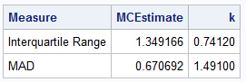
The Monte Carlo estimates from the simulation are very close to the theoretical values:

For the IQR statistic, the average value is approximately 1.3492. The reciprocal is 0.7412, which is close to the true theoretical value 0.7413.
For the MAD statistic, the average value is approximately 0.6707. The reciprocal is 1.4910, which is close to the true theoretical value 1.4826.

Extending the simulation to other measures of dispersion

For any statistical measure of scale, you can use a Monte Carlo simulation to estimate the constant for which the statistic becomes a consistent estimator of the standard deviation: Generate many random samples from N(0,1), compute the statistic on each sample, and compute k = 1/MCAvg, where MCAvg is the mean of the Monte Carlo statistics. This is a practical method to produce a consistent estimator even if the theoretical distribution of the statistic is unknown or very complicated.

You can also use this method to produce consistent estimators when the data are not normal. You would need to change the simulation to sample from a nonnormal distribution.

Summary

When you use the ROBUSTSCALE option in PROC UNIVARIATE, SAS automatically scales these robust statistics to produce a consistent estimator for the standard deviation of normally distributed data. The scaling factors are derived by using theoretical computations. (See the Appendix.) By using a Monte Carlo simulation, we can understand the significance of these multiplicative constants. They are the factors that make the expected value of a robust statistic equal to the standard deviation of a normal distribution.

Appendix: The scaling factors for MAD and IQR

A Wikipedia article about robust statistics derives the scaling factors for the MAD and IQR statistics. For normal data, the expected value of the MAD statistics is Φ^-1(0.75), where Φ is the standard normal CDF. The expected value for the IQR statistic is Φ^-1(0.75) – Φ^-1(0.25). Therefore the following DATA step computes the exact multiplicative factors for MAD and IQR to be consistent estimators:

data Rescale;
Statistic = "IQR";
Expected = quantile("Normal", 0.75) - quantile("Normal", 0.25);
k = 1 / Expected;
output;
Statistic = "MAD";
Expected = quantile("Normal", 0.75);
k = 1 / Expected;
output;
format _numeric_ 6.4;
run;
 
proc print data=Rescale noobs;
run;

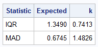
Notice that the IQR is exactly twice the MAD for the normal distribution.

Blogs