In statistical quality control, practitioners often estimate the variability of products that are being produced in a manufacturing plant. It is important to estimate the variability as soon as possible, which means trying to obtain an estimate from a small sample. Samples of size five or less are not uncommon in manufacturing, especially it each item is expensive or takes a long time to manufacture.

Quality control practitioners sometimes choose to use the sample range to estimate the variability from a very small samples. The range (the maximum value minus the minimum value) is a robust statistic, and it is trivial to compute a sample range in your head as products roll off the assembly line. But many statisticians do not have an intuitive feel for ranges. Statisticians are more familiar with the standard deviation. But fear not! Remarkably, when the underlying measurements are normally distributed, there is a constant (that depends on the sample size) that enables you to estimate the standard deviation of a process from a measurement of the sample range! Thus, you can essentially "convert" a range measurement into an estimate for the standard deviation.

The conversion constant is named d2, or d2(n) if you want to emphasize the dependence on the sample size. SAS provides the D2 function as part of SAS/QC software. The D2 function computes the d2 constant for 2 ≤ n ≤ 25. For larger samples, the standard deviation or MAD statistic is a more efficient estimate of variability. This article discusses the d2 constant, how to compute it, and how to use it to estimate the standard deviation in small normally distributed samples. The Appendix shows that if you do not have SAS/QC software, you can compute d2 by evaluating a complicated integral on an infinite domain.

The expected value of the range in small normal samples

The d2 constant is defined as the expected value of the range statistic in a random sample of size n that is drawn from a normal distribution. You can run a simulation to better understand concepts like the expected value of a statistic. I will use PROC IML for the simulation because I also want to show how to use PROC IML to compute d2 by evaluating an integral.

The following SAS IML statements simulate one sample of size n=5 from the standard normal distribution. I could use the RANGE function to compute the range statistic, but in preparation for the simulation study, I will use the column-wise subscript reduction operators to compute the maximum and minimum values of each column, then form the range from those statistics. First, generate one sample of size n=5:

%let SampleSize = 5;       /* the D2 constant is defined for 2 <= n <= 25 */
proc iml;
call randseed(1234);       /* set random number seed */
n = &SampleSize;           /* n = sample size */
x = j(n,1);
call randgen(x, "Normal"); /* x ~ N(0,1) */
min = x[><];               /* max(x) */
max = x[<>];               /* min(x) */
OneRange = max - min;
print min max OneRange;

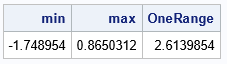
For this random sample, the maximum data value is 0.865 and the minimum value is -1.749. Therefore, the sample range is 2.614. Of course, the range will be different for each random sample, so let's next simulate 10,000 random samples and look at the distribution of the ranges:

/* Monte Carlo simulation: Plot the distribution of the range statistic */
nSamples = 10000;          /* create 10,000 random samples */
x = j(n, nSamples);        /* each column is sample is size n */
call randgen(x, "Normal"); /* x ~ N(0,1) */
min = x[><, ];             /* max of each column */
max = x[<>, ];             /* min of each column */
range = max - min;       
 
title "Distribution of Sample Range";
title2 "Normal Samples, n=&SampleSize";
call histogram(range);

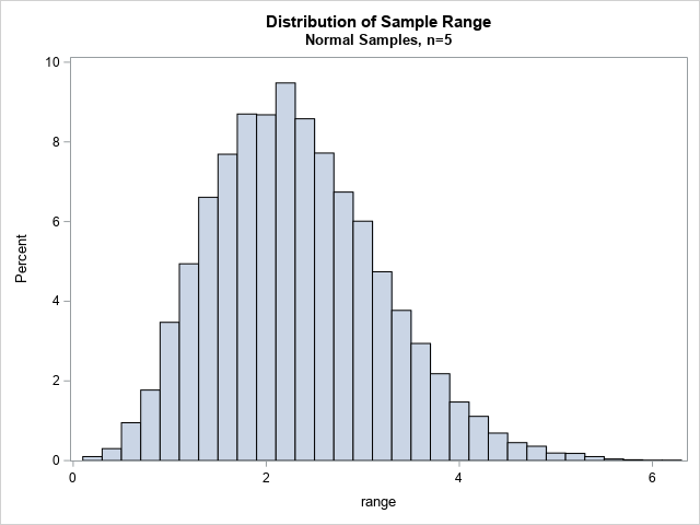
The histogram shows the Monte Carlo distribution of the sample range. In some samples, the range was barely positive. In other samples, the range was as large as 6 units. The most common sample range is about 2.3.

You can estimate the expected value of this distribution by using the mean of the Monte Carlo statistics, as shown by the following statements:

/* What is the expected value of the range in a normal sample of size n? */
/* Use Monte Carlo average to estimate the expected value */
MCEst = mean(colvec(range));
print MCEst;

The Monte Carlo estimate of the expected value is approximate 2.32. That estimate depends on the number of Monte Carlo samples and the specified value of the random number seed.

The d2 constant

As mentioned earlier, you don't need to run a Monte Carlo simulation to obtain the expected value of the sample range in a standard normal sample of size n. SAS provides the D2 function. The value d2(n) for 2 ≤ n ≤ 25 is the expected value for the range in a sample of size n. The following call evaluates the exact d2 value and compares it to the Monte Carlo estimate:

d2 = d2(n);      /* d2 = E(range; n=5). The D2 function is defined in SAS/QC software */
print MCEst d2 (MCEst/d2)[L="Ratio"] ;

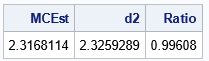
The output shows that the Monte Carlo estimate is close to the exact value. The ratio of the two quantities is approximately 1.

Use the range to estimate the standard deviation

As discussed in the documentation for the D2 function, you can use the d2 constant to estimate the standard deviation from the range. The documentation states, "you can use the constant d2 to calculate an unbiased estimate of the standard deviation (sigma) of a normal distribution from the sample range of n observations." It then says that the quantity (Sample Range) / d2(n) is an estimate for the standard deviation in a normal sample. So, the following histogram shows the estimated the distribution of the sample standard deviation in the Monte Carlo samples. Furthermore, the ratio (MCEst / d2) ≈ 0.996 is a Monte Carlo estimate of the standard deviation. Recall that we simulated the data from a standard normal distribution, so the estimate is very close to 1, which is the true value.

/* an estimate of sigma in each sample is (sample range) / d2(n) */
SDEstFromRange = range / d2;
 
title "Approximate Distribution of Standard Deviation";
title2 "(Sample Range) / d2(n), n=&SampleSize";
call histogram(SDEstFromRange) grid={x y} label="Range / d2";

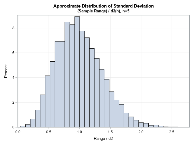
The histogram shows an approximate distribution for the sample standard deviation in these samples. This distribution looks reasonable because the samples are from a N(0,1) distribution, and the distribution shows a pronounced peak near 1. Many statisticians are more comfortable interpreting the statistical deviation than the range statistic.

The true relationship between the range and the standard deviation

Of course, you could use the usual sum-of-squares formula to estimate the standard deviation for each sample. To demonstrate that the usual estimate of the standard deviation is close to the scaled range, compute the standard deviation for each of the 10,000 samples. Then plot the standard deviations and the scaled ranges against each other, as follows:

sd = std(x);               /* std deviation for each sample */
title "Scaled Range and Standard Deviation in Normal Samples";
title2 "n = &SampleSize";
call scatter(SDEstFromRange, sd) grid={x y} procopt="noautolegend"
             option="transparency=0.9" label={'(Sample Range) / D2', 'StdDev'}
             other="lineparm x=0 y=0 slope=1 / lineattrs=(color=red);";

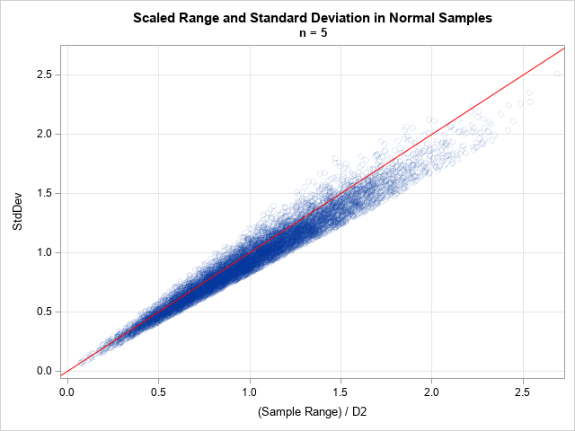
The markers in the scatter plot are all close to the diagonal identity line (y=x), which shows that the range divided by d2 is a good estimate for the standard deviation for every sample.

Summary

Quality control practitioners sometimes use the sample range to estimate of variability in very small samples. When the underlying measurements are normally distributed, you can "convert" a range measurement into an estimate for the standard deviation. The d2 constant (which depends on the sample size) is the expected value of the sample range. It enables you to estimate the standard deviation of a process from a measurement of the sample range.

Appendix: Compute d2 by solving an integral

Although the D2 function is built into SAS/QC software, it is instructive to compute the d2 constant from its definition. The d2 constant is defined by an integral:

Whenever you see an expression like (1 - Φ(x)) for a right-tailed probability, you should use the SDF function rather than the CDF function. Therefore, the following SAS IML functions define the integrand and an alternative to the built-in d2(n) function:

proc iml;
/* Although the D2 function is supported in SAS/QC, 
   you can also compute d2 by evaluating an improper integral */
start D2Integrand(x) global(g_n);
   n = g_n;
   return( 1 - SDF("Normal",x)##n - CDF("Normal",x)##n );
finish;
 
/* integrate the function on (-Infinity, Infinity) */
start D2Integral(n) global(g_n);
   interval = {.M .P};
   g_n = n;
   call quad(d2, "D2Integrand", interval);
   return( d2 );
finish;
 
n = 5;
altD2 = D2Integral(n);
d2 = d2(n);
print altD2 d2 (d2-altD2)[L="Diff"];

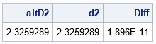
As promised, evaluating the interval on the infinite domain results in the same value as the built-in D2 function in SAS.