A previous article shows how to compute various robust estimates of scale in SAS. In that article, I show how to scale these robust estimators so that they become consistent estimators of the standard deviation (σ) when the data are normally distributed. The scaling factor is related to the expected value of the statistics for normal data.

The range is also a measure of dispersion, although it is not robust to outliers. I have previously shown how to use the range to form a consistent estimator of σ for normally distributed data. The scaling factor depends on the expected value of the range for a normal sample of size n, which is called d₂(n).

When the sample size is small (n ≤ 25), quality control engineers use the range to estimate the standard deviation. You can find values of d₂(n) in a table or use the previous article to compute values by using the D2 function in SAS/QC software or by solving an integral by using SAS IML.

I recently saw an approximation to d₂(n) by using an asymptotic (large n) formula. An asymptotic formula approximates the expected value of the range in a normal sample when n is large. I was surprised to discover that the asymptotic approximation is not a good approximation for d₂(n) for moderately large samples, such as n < 1000. This post compares the asymptotic formula to the exact value of d₂(n) and compares both methods with a Monte Carlo simulation.

The Expected Range and Extreme Value Theory

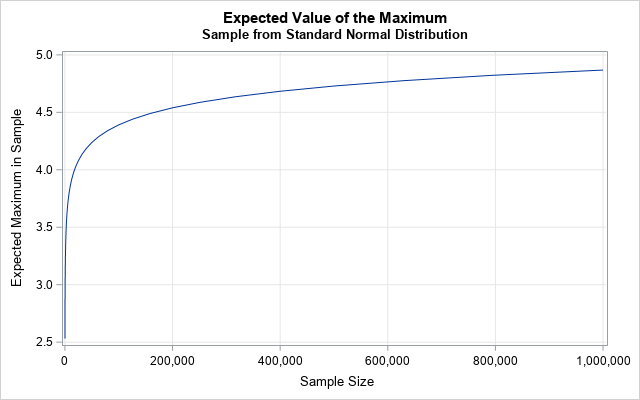
The range of a sample is the difference between the maximum and the minimum values: R = X_(n) - X₍₁₎. For a symmetric distribution like the normal distribution, the expected value of the range is simply twice the expected value of the maximum: E[R] = 2·E[X_(n)].

I have previously shown that as n becomes large, the distribution of the maximum of a normal sample approaches a Gumbel distribution. The graph of the expected value of the maximum is shown to the left for large sample sizes. You can write down formulas that describe the asymptotic behavior of this function. I used formulas in David and Nagaraja (2004, Order Statistics, 3rd Ed.). First, define the following functions:

• $s_n = \sqrt{2 \log n}$
• $b_n = s_n - \frac{\log(\log n) + \log(4\pi)}{2s_n}$
• $a_n = \frac{1}{s_n}$

In these formulas, LOG is the natural logarithm. By using these expressions, you can construct several asymptotic approximations for d₂(n). Each approximation adds one additional term to the previous approximation:

1. 1-term approximation: 2s_n. This is the simplest (and crudest) estimate.
2. 2-term approximation: 2b_n. This a better approximation, but it tends to underestimate d₂(n).
3. 3-term approximation: 2(b_n + γa_n), where γ ≈ 0.5772 is the Euler-Mascheroni constant. This accounts for the fact that the mean of the limiting Gumbel distribution is γ. This is the best approximation of the three.

These are large-n approximations for d₂(n). The following SAS DATA step compares the exact values of d₂(n) to these asymptotic formulas.

/* d2(n) is the scale factor to use to adjust the range statistic so that 
   it is a consistent estimator of the standard deviation for normal data.
   Some references use asymptotic approximations for d2(n).
   Define the formulas 
   sn = sqrt(2*log(n));
   bn = sn - (log(log(n)) + log(4*pi)) / (2*sqrt(2*log(n)));
   an = 1 / sn;
 
   Then the following are 1-term, 2-term, and 3-term asymptotic approximations for d2(n):
 
   Number of Terms    Formula
   1 term             2 * sn
   2 terms            2 * bn
   3 terms            2 * (bn + gamma*an), where gamma~0.57721... is the Euler-Mascheroni constant
*/
data k_n;
/* Compute or look up the value of d2(n) in a table for certain values of n.
   Compare those exact values to several asymptotic (large n) approximations. */
array nA[5]   _temporary_ (2,      50,     100,    500,    1000);
array d_nA[5] _temporary_ (1.1284, 4.4982, 5.0151, 6.0734, 6.4829);
pi = constant('pi');
gamma = constant('Euler');  /* 0.57721... */
do i = 1 to dim(nA);
   n  = nA[i];
   d2_n = d_nA[i];
   sn = sqrt(2*log(n));
   bn = sn - (log(log(n)) + log(4*pi)) / (2*sqrt(2*log(n)));
   an = 1 / sn;
   Asymp1 = 2 * sn;
   Asymp2 = 2 * bn;
   Asymp3 = 2 * (bn + gamma*an);
   output;
end;
drop pi gamma i sn bn an;
run;
 
proc print data=k_n noobs; 
   format _all_ best5.; 
   ID n; 
run;

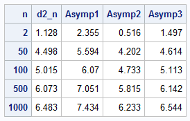
I have seen researchers use these asymptotic approximations for values of n as small as 50 or 100. But, as you can see, the approximations are not close to d₂(n) for those values of n. In fact, David and Nagaraja (2003) warn that these asymptotic approximations converge quite slowly. Even at n = 1000, the approximations are not very close to the true value. I do not recommend these asymptotic approximations for small or moderate sample sizes.

Testing the Estimators: A Monte Carlo Simulation

You can run a Monte Carlo simulation to estimate d₂(n), which is the expected range of a normal sample of size n. The following SAS DATA step generates 1,000 samples of size n = 100 from a standard normal distribution. For each sample, PROC MEANS calculates the range. In a second DATA step, the range is divided by three different factors: the exact d₂(100), the 2-term approximation, and the 3-term approximation. These "adjusted ranges" are the various estimates for the standard deviation, which is 1 for this simulation. I do not show the 1-term adjusted range because it is so bad.

/* simulate 1000 random samples of size n=100 from N(0,1) */
%let N = 100;
%let numSamples = 1000;
data SimNormal;
call streaminit(12345);
do sampleID = 1 to &numSamples;
   do i = 1 to &n;
      x = rand("Normal");
      output;
   end;
end;
keep sampleID x;
run;
 
/* compute the range for each random sample */
proc means data=SimNormal noprint;
    by sampleID;
    var x;
    output out=RangeOut RANGE=Range;
run;
 
/* adjust the range statistics by using d2(100), Asymp2, or Asymp3 formula */
data AdjustRange;
pi = constant('pi');
gamma = constant('Euler');  /* 0.5772156649 */
set RangeOut(rename=(_FREQ_=n));
d2_n = 5.0151;
sn = sqrt(2*log(n));
bn = sn - (log(log(n)) + log(4*pi)) / (2*sqrt(2*log(n)));
an = 1 / sn;
Asymp2 = 2 * bn;
Asymp3 = 2 * (bn + gamma*an);
 
AdjRange_d2     = 1/d2_n   * Range;
AdjRange_2Term  = 1/Asymp2 * Range;
AdjRange_3Term  = 1/Asymp3 * Range;
keep SampleID Range AdjRange_d2 AdjRange_2Term AdjRange_3Term;
label AdjRange_d2="d2" AdjRange_2Term="2-Term Asymptotic" AdjRange_3Term="3-Term Asymptotic";
run;
 
/* Print the Monte Carlo estimates of the adjusted range, which should be close to sigma=1.
   Note that the 95% CI for the mean includes 1 for d2(100), but not for the asymptotic approx. 
*/
proc means data=AdjustRange Mean CLM ndec=3 nolabels;
   var AdjRange_d2 AdjRange_2Term AdjRange_3Term;
run;

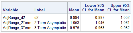
Since the data were generated from N(0,1), a consistent estimator should produce an average value close to 1.0. The results show that the Monte Carlo estimate is consistent if you use the d₂(100) value to scale the data. For the asymptotic formulas, you get biased estimates. The two-term asymptotic approximation overestimates the standard deviation whereas the two-term asymptotic approximation underestimates it. These results are reproducible: they do not change if you use additional Monte Carlo trials.

Summary

The expected range of normal data is a quantity known as d₂(n). This article shows several asymptotic approximations. The asymptotic approximations provide a simple expression that you can use to predict the range in a very large random sample of normal data. However, these estimates converge quite slowly. In quality control, the range is used to estimate the standard deviation of normal data when n is small. You should not use the asymptotic approximations of d₂(n) for that purpose.