Visualize a multivariate regression model when using spline effects

A SAS analyst read my previous article about visualizing the predicted values for a regression model that uses spline effects. Because the original explanatory variable does not appear in the model, the analyst had several questions:

How do you score the model on new data?
The previous example has only one explanatory variable. How do you score a model that has additional continuous or categorical covariates?
How do you create a plot that shows the fit plotted against the original explanatory variable?

This article explains how to score the model on new data and how to visualize the predicted values by plotting them against the explanatory variable that you used to generate the spline effects. Although the model uses spline effects, everything in this article also applies to models that do not use splines.

A naïve visualization of a multivariate regression model

I have previously discussed how to use the EFFECT statement in SAS regression procedures to build regression models that use cubic splines to model nonlinear relationships between the response variable and an explanatory variable. For procedures that do not support an EFFECT statement, you can write the spline basis functions to a data set and then use those effects as explanatory variables in a model.

Visualizing a regression model that has multiple covariates can be a challenge because the "obvious" visualization does not work! The "obvious" (but wrong!) visualization uses an OUTPUT statement to write the predicted values to a data set, then plots the predicted values versus one of the continuous variables. But the following example shows that this naïve approach does not give you an effective visualization when there are multiple covariates:

/* sort the data and choose a subset of 4-, 6-, and 8-cylinder vehicles */
proc sort data=sashelp.cars out=cars(Where=(Type^="Hybrid" and Cylinders in (4,6,8)));
   by  EngineSize;
run;
 
/* Fit data by using restricted cubic splines.
   The EFFECT statement is supported by many procedures: GLIMMIX, GLMSELECT, LOGISTIC, PHREG, ... 
*/
proc glmselect data=cars;
   effect spl = spline(EngineSize / details       /* define spline effects */
                naturalcubic basis=tpf(noint)     /* natural cubic splines, omit constant effect */
                knotmethod=equal(4));             /* 4 evenly spaced interior knots */
   class Cylinders;
   model mpg_city = spl Cylinders Weight / selection=none;  /* include categorical and continuous covariates */
   output out=GLSOut pred=p_MPG_City;             /* try to use predicted values on original data */
quit;
 
title "Predicted Values at Data Values from OUTPUT Statement";
title2 "This Output Is Not Useful!";
proc sgplot data=GLSOut;
   scatter x=EngineSize y=MPG_City;
   series x=EngineSize y=p_MPG_City / group=Cylinders;
   xaxis grid;
   yaxis grid label="Predicted MPG (City)";
run;

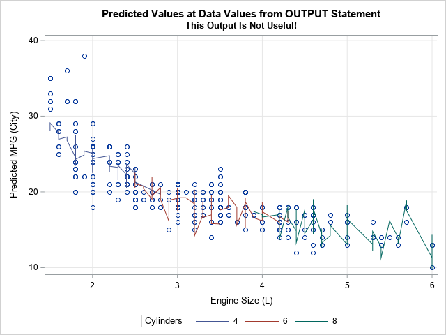
This graph looks strange, but the strangeness is not because the model uses splines. Every multivariate regression model will look similar when you project the predicted values onto one of the covariates. The reason that two observations that have the same (or nearly the same) value for the horizontal variable in the graph (EngineSize, in this example) might have very different values in one of the other covariates. This means that for every horizontal value, there are multiple response values. Consequently, when you use a SERIES statement to plot the predicted values, the line looks jagged as it traces out multiple Y values for each X value.

You can see the range of predicted values by using PROC PRINT. The following statements display the predicted values for observations at the extreme right edge of the graph:

proc print data=GLSOut;
   where EngineSize=6.0;
   var Make Model EngineSize Cylinders Weight MPG_City p_MPG_City;
run;

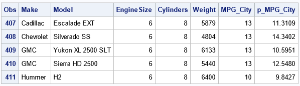
The table shows that the Weight values are different for the five vehicles that have 6.0-liter engines. Because the Weight variable is included in the model, the predicted values are also different. Thus, when EngineSize=6, the SERIES statement draws a vertical segment that spans the range [9.84, 14.34] in the vertical direction. The same explanation is valid for other values of EngineSize, which leads to the jagged line.

The sliced plot: A better visualization of a multivariate regression model

The solution to this problem is to use a sliced fit plot. In a sliced fit plot, you evaluate the model at the following set of points:

For the variable that you are plotting, evaluate the model on a regular grid of values. In this example, you might choose the values 1.5 to 6.0 in steps of 0.1 for the EngineSize variable because the minimum (respectively, maximum) value of the variable in the data is 1.5L (respectively, 6.0L).
For the covariates, choose a representative variable. For continuous covariates, this is often a mean or median value; For categorical covariates, this is often a mode or the reference level. In this example, you might choose the value 3,500 pounds for the Weight variable because that is a "round" value close to the mean and median weight. You might choose 6 as a value for the Cylinders variable, since a 6-cylinder car is a very common vehicle.
There might be situations where you want to overlay two or more curves on a scatter plot, where the curves represent the model evaluated at multiple values of a categorical variable. In this example, you might want to see separate curves for 4-, 6-, and 8-cylinder vehicles.

The good news is that there is a straightforward way to obtain a sliced fit plot in SAS! Many SAS regression procedures support the STORE statement, which enables you to create an item store for the model. You can use the EFFECTPLOT statement in PROC PLM to create a sliced fit plot. For more control over the visualization, you can use the SCORE statement in PROC PLM to evaluate the model at any set of points that you want.

This works because the item store contains not only the parameter estimates for the spline basis, but also the transformation that generates the spline effects from the original explanatory variable.

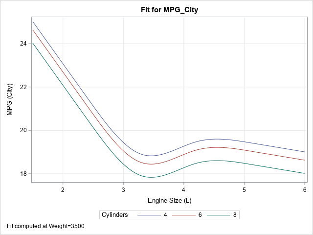
For example, the following model includes spline effects. The program uses the STORE statement to save the model to an item store, then uses PROC PLM to plot the predicted values against the EngineSize variable for various values of the covariates:

proc glmselect data=cars;
   effect spl = spline(EngineSize / details       /* define spline effects */
                naturalcubic basis=tpf(noint)     /* natural cubic splines, omit constant effect */
                knotmethod=equal(4));             /* 4 evenly spaced interior knots */
   class Cylinders Origin;
   model mpg_city = spl Cylinders Weight / selection=none;  /* include categorical and continuous covariates */
   store out=GLSModel;
run;
 
title "Predicted Values at Specified Values from PROC PLM";
title2 "Model Uses Splines";
proc plm restore=GLSModel;
   effectplot slicefit(x=EngineSize sliceby=Cylinders) / at(Weight=3500); 
run;

Notice the information that you can supply to the SLICEFIT keyword in the EFFECTPLOT statement:

The X= suboption specifies the horizontal variable for the sliced fit plot. If you omit this option, the first continuous variable in the model is used.
The SLICEBY= suboption specifies a CLASS variable. The plot will overlay curves for each level of the SLICEBY= variable. If you omit this option, the first CLASS variable is used.
AT option on the EFFECTPLOT statement enables you to specify a list of variable-value pairs for evaluating the model. If you omit this option, each continuous covariate is evaluated at its mean value, and CLASS variables are evaluated at their reference level. You can specify a list of variable-value pairs. For example, if you create a model with additional covariates, you could specify AT(Origin='Asia' Weight=3500 HorsePower=300).

Scoring a multivariate regression model

PROC PLM is also useful to scoring the model on a new set of data is straightforward. This is sometimes necessary when you want complete control over the values at which to evaluate the model. To score the model at arbitrary locations, generate the scoring data and use the SCORE statement in PROC PLM, as follows:

/* Create a scoring data set. 
   For cars, mean(Weight)=3570 and median(Weight)=3473, so use 3500 as "round" value. */
data ScoreIn;
   Weight = 3500;        /* a value close to the mean */
   do Cylinders = 4,6,8; /* important modes */
      do EngineSize = 1.5 to 6 by 0.1;
         output;
      end;
   end;
run;
 
/* score the model by using PROC PLM */
proc plm restore=GLSModel;
   score data=ScoreIn out=ScoreOut;
quit;

You can use the ScoreOut data set to create your own sliced fit plot by using PROC SGPLOT. Scoring the data enables you to overlay observations, add labels, and enhance the plot in other ways. For example, you can combine the predicted values with the original data and overlay them, as follows:

/* you can combine the original data and the predicted value to visualize the sliced model */
data Combine;
   set cars
       ScoreOut(rename=(          
          Weight = scoreWeight
          Cylinders = scoreCylinders
          EngineSize = scoreEngineSize ));
run;
 
title "Model Scored at Weight=3500";
proc sgplot data=Combine;
   scatter x=EngineSize y=MPG_City / markerattrs=(symbol=CircleFilled) colorresponse=Weight colormodel=(yellow red);
   series x=scoreEngineSize y=Predicted / group=scoreCylinders name="pred" nomissinggroup;
   xaxis grid;
   yaxis grid label="MPG (City)";
   gradlegend / position=bottom;
   keylegend "pred" / title="Cylinders" across=1 position=right;
run;

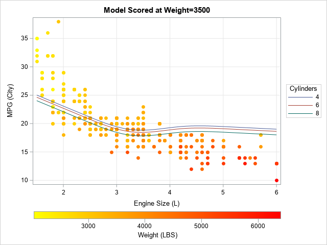
This graph shows a potential pitfall of evaluating a model at the mean or median of a covariate. For these data, the EngineSize and Weight variables are highly correlated (r=0.83). A consequence of that fact is that small vehicles tend have small engines and small weights; large vehicles tend to have large engines and large weights. (There are also sports cars, which have large engines and small weights.) When you evaluate the model at the value Weight=3500 and overlay the predicted values on the data, the fit does not seem to pass through the bulk of the data. It under-predicts the MPG for small cars and over-predicts the MPG for large cars. This happens because many vehicles have weights that are far from 3,500 pounds. You should not expect the predicted MPG_City (which is for reference value, Weight=3500) to be close to the observed MPG_City when the observed weight is far from the reference value.

Summary

This article shows how to use the EFFECTPLOT statement in PROC PLM to visualize multivariate regression models, with an emphasis on models that include spline effects. The EFFECTPLOT SLICEFIT statement enables you to specify the variable to use for the X axis, and the value of the covariates at to evaluate the model. Optionally, you can specify a classification variable and get several curves, one for each level of the classification variable.

In a similar way, you can use the SCORE statement in PROC PLM to evaluate the model at an arbitrary set of values for the explanatory variable. When used correctly and in conjunction with PROC SGPLOT, this gives you absolute control over the visualization of multivariate regression models.

The ideas in this article also apply to models that do NOT use spline effects.

Blogs