I read a journal article in which a researcher used a formula for the probability density function (PDF) of the sample correlation coefficient. The formula was rather complicated, and presented with no citation, so I was curious to learn more. I found the distribution for the correlation coefficient in the classic reference book, Continuous Univariate Distributions (Johnson, Kotz, and Balakrishnan, 1995, 2nd Ed), and discovered that there are six (!) known formulas for the PDF of the correlation coefficient, assuming that the correlation is for a random sample of size n drawn from a bivariate normal distribution with correlation ρ. (Notice the normality assumption.) From a computational perspective, two seemed straightforward to implement in SAS.
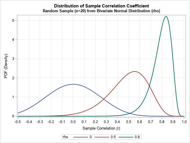
This article shows how to implement a function that evaluates the PDF of the correlation in a random sample of size n when the sample is drawn from a bivariate normal distribution. The PDF has the form f(r; ρ, n), which means that it is a function of r (-1 ≤ r ≤ 1) and depends on the sample size, n, and the underlying normal correlation, ρ. To whet your appetite, the graph at the right shows the distribution of the sample correlation in bivariate normal samples of size n = 20, where the underlying correlation is ρ = 0, 0.5, and 0.8.
A formula that evaluates an improper integral
The formula that I saw in the journal article is shown below. The image is scanned from Eqn. 32.6b on p. 549 of Johnson, Kotz, and Balakrishnan (1995):
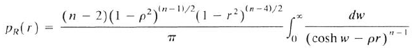
Apparently, this formula was discovered by Fisher about 100 years ago! This formula enables you to evaluate the probability density function for the sample correlation (r) when the sample size (n) and the underlying bivariate correlation (ρ) are supplied. The challenging part of the formula is evaluating the improper integral. The dummy variable is w, so n, r and ρ are constants when performing the integration.
Is the integral hard to compute? Well, recall that the hyperbolic cosine, cosh(w), is asymptotic to exp(w) for large values of w. Since -1 ≤ ρr ≤ 1, the integrand is asymptotically approaching exp(-(n-1)w), which decays very quickly and implies that the integral on (0, ∞) might decay quickly and be relatively easy to compute.
You can numerically integrate integrals by using the QUAD function in SAS IML software. The infinite interval is defined by using the special missing value, .P, to indicate positive infinity, as follows:
proc iml; /* Integrand is 1 / (cosh(w) - r*rho)##(n-1) = (cosh(w) - r*rho)##-(n-1) Specify constants as GLOBAL variables prefixed by 'g_'. */ start Integrand(w) global(g_r, g_rho, g_n); return (cosh(w) - g_r*g_rho)##(-(g_n-1)); finish; /* set parameters for an example */ n = 20; rho = 0.6; /* define the global variables and integrate the function on (0, Infinity) */ g_r = 0.5; g_rho = rho; g_n = n; domain = {0 .P}; /* (0, Infinity) */ call quad(integral, "Integrand", domain); print integral; |

I do not know the derivation of the formula, so I don't know what this integral represents. However, you can use it to implement Fisher's formula for the PDF of the sampling distribution of the correlation coefficient. Notice that the SAS IML language enables you to implement the complicated formula by using a readable syntax:
start CorrPDFFisher(r, rho, n) global(g_r, g_rho, g_n); /* copy values to global vars for the integration */ g_r = r; g_rho = rho; g_n = n; domain = {0 .P}; call quad(integral, "Integrand", domain); /* compute the integral */ pi = constant('pi'); C = (n-2) * (1-rho**2)##((n-1)/2) * (1-r**2)##((n-4)/2) / pi; return C*integral; finish; /* evaluate the PDF for a range of r values and graph the PDF */ r = do(-0.2, 1, 0.01); PDF = j(1, ncol(r), .); do i = 1 to ncol(r); PDF[i] = CorrPDFFisher(r[i], rho, n ); end; title "Distribution of Sample Correlation Coefficient"; title2 "rho = 0.6; n = 20; Fisher's Formula"; call series(r, PDF) grid={x y}; |
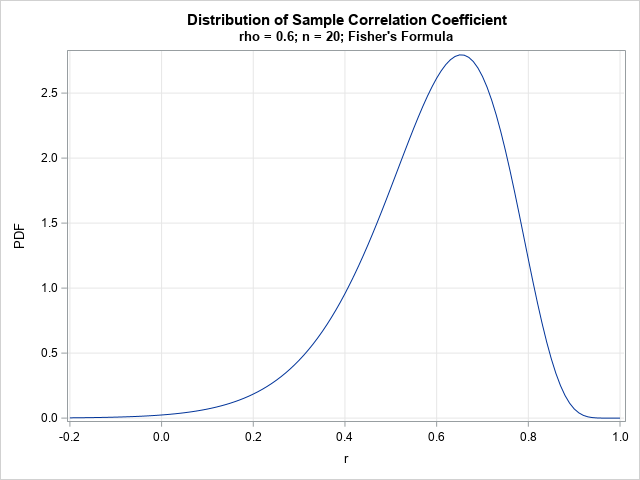
The graph shows the sampling distribution of the Pearson correlation statistic in a random sample of size n=20 that is drawn from bivariate normal data with correlation ρ=0.6. Notice that the probability of getting a statistic that is negative is small, as is the probability of getting a value near 1. Most statistics will be the range [0.4, 0.8] with values near 0.65 being most likely. It is interesting that the most likely statistic is 0.65 even though the underlying correlation in the population is ρ=0.6. The expected value of the sample correlation is approximately 0.59, which indicates that the statistic is a biased estimator of the underlying correlation parameter (Fisher, 1915). Fortunately, this bias is small (on the order of 1/n) and is negligible for large samples.
The exact formula for the PDF enables you to compute other statistics, such as exact confidence intervals. However, in practice the confidence intervals are usually computed by using Fisher z-transform, which transforms the (skewed) distribution of the sample correlation into a normal distribution. For example, in PROC CORR, you can use the FISHER option to obtain confidence intervals based on Fisher's transformation.
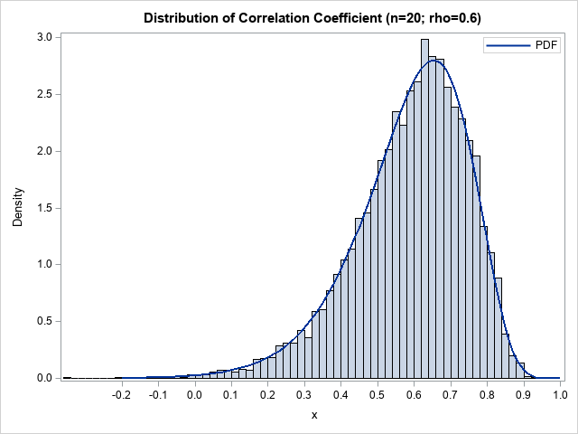
How do we know that this graph is correct? A common way to validate a PDF computation is to overlay the curve on a histogram of statistics that are computed as part of a large simulation. For example, you can simulate 10,000 random bivariate normal samples of size n=20 and compute the correlation for each sample. You can then plot the distribution of the sample correlations by using a histogram. (Or, even better, use the Wishart distribution to simulate the correlation coefficients directly!) The following graph overlays the simulated distribution and the exact PDF:
The distribution for other parameter values
The previous section shows how to compute the density function for the sample correlation for specified values of n and ρ. Of course, you can vary these parameters from the values in the previous section. For example, the following SAS IML statements compute the density function for three values of ρ in bivariate normal samples of size n=20:
/* let's draw the PDF for rho = 0, 0.5, and 0.8 */ rhoVec = {0 0.5 0.8}; n = 20; r = do(-0.5, 1, 0.01); PDF = j(1, ncol(r), .); results = {. . .}; create CorrPDF from results[c={'rho' 'r' 'PDF'}]; do j = 1 to ncol(rhoVec); rho = rhoVec[j]; do i = 1 to ncol(r); PDF[i] = CorrPDFFisher(r[i], rho, n ); end; results = j(ncol(r), 1, rho) || r` || PDF`; append from results; end; close; QUIT; title "Distribution of Sample Correlation Coefficient"; title2 "Random Sample (n=20) from Bivariate Normal Distribution (rho)"; proc sgplot data=CorrPDF; series x=r y=PDF / group=rho lineattrs=(thickness=2); xaxis grid values=(-1 to 1 by 0.1) valueshint label="Sample Correlation (r)"; yaxis grid label="PDF (Density)"; run; |
The graph is shown at the top of this article. The distribution for ρ=0 is symmetric. For ρ > 0, you can see that the distribution is skewed; the mode is to the right of the expected value.
Other formulas for the exact distribution
Johnson, Kotz, and Balakrishnan (1995) show six different formulas for the exact distribution of the sample correlation in bivariate normal samples. Another that is often used is by Hotelling (1953). The following image is scanned from Eqn. 32.6e on p. 549:
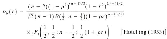
This formula is equivalent to the formula in the Wikipedia article for the Pearson correlation coefficient. It uses Gauss's hypergeometric function (denoted \(\,_2F_1\)). I have previously shown how to evaluate Gauss's hypergeometric function in SAS. I won't reproduce the full analysis here, but you can download the complete SAS IML program from GitHub.
Summary
This article shows how to evaluate a complicated formula for the PDF of the correlation coefficient in bivariate normal samples. The formula requires evaluating an integral on an infinite domain. Despite the complexity, evaluating the function requires only a dozen statements in the SAS IML language. You can download the SAS program that evaluates the function and creates the graphs in this article. I also include a second function that evaluates the PDF by using a different formula that requires evaluating a hypergeometric function.
