Compute hypergeometric functions in SAS

In applied mathematics, there is a large collection of "special functions." These function appera in certain applications, often as the solution to a differential equation, but also in the definition of probability distributions. For example, I have written about Bessel functions, the complete and incomplete gamma function, and the complete and incomplete beta function, and the Lambert W function, just to name a few special functions that are encountered in statistics.

You can be blissfully ignorant of a special function for many years, then one day you encounter a problem in which the function is essential. This happened recently when a SAS programmer told me about a problem that requires computing with a two-dimensional hypergeometric function. I had never heard of the function, but I did some research to figure out how to compute the function in SAS. (For a mathematical overview, see Beukers, 2014.) This article shows how to use numerical integration in SAS to compute a one-dimensional hypergeometric function, which is called Gauss's hypergeometric function and denoted $\,_2F_1$ . A subsequent article will discuss a two-dimensional hypergeometric function, which is needed to compute the PDF of a certain probability distribution. I am not an expert on the hypergeometric function, but this article shares what I have learned.

Hypergeometric functions are sometimes defined as functions of complex numbers, but the applications in statistics involve only real numbers. Consequently, this article evaluates the functions for real arguments. The hypergeometric functions in this article converge when the magnitude of each variable is less than 1.

A one-dimensional hypergeometric function

For the definition of Gauss's hypergeometric function, see the Wikipedia article about the 1-D hypergeometric series. Hypergeometric functions are defined as an infinite series. The one-dimensional hypergeometric functions have three parameters, (a,b;c). The most useful hypergeometric series is denoted by $\,_{2}F_{1}(a,b;c; x)$ or sometimes just as $F(a,b;c; x)$ , where |x| < 1. Interestingly, the convention for a hypergeometric function is to list the parameters first and the variable (x) last. The two parameters (a,b) are called the upper parameters; the parameter c is called the lower parameter. The $\,_2F_1$ function is a special case of the generalized hypergeometric function $\,_pF_q$ , which has p upper parameters and q lower parameters.

Compute Gauss's hypergeometric function in SAS

An important special case of the parameters is c > b > 0 and a > 0. If c > b > 0, then you can write the hypergeometric function as a definite integral. The defining equation is
$B(b,c-b) * \,_{2}F_{1}(a,b;c; x)=\int _{0}^{1}u^{b-1}(1-u)^{c-b-1} / (1-x u)^{a}\,du$
where B(s,t) is the complete beta function, which is available in SAS by using the BETA function. Both arguments to the BETA function must be positive, so evaluating the BETA function requires that c > b > 0. Notice that the integration variable, u, does not appear in the answer. The definite integral is a function of the parameters (a,b,c) and of the variable x.

You can perform numerical integration in SAS by using the QUAD function in SAS IML software. Notice that when a > 0, the integrand becomes unbounded as x → 1. Because of this, the QUAD function will display some warnings in the log as it seeks an accurate solution. According to my tests, the value of this integral seems to be computed correctly.

The following SAS IML program uses the QUAD function to evaluate the definite integral by using the user-defined HG1 function. The GLOBAL statement enables you to pass values of the parameters (a,b,c) and the variable x. I use G_ as a prefix to denote global variables. After evaluating the integral for each value of x, the function Hypergeometric2F1 divides the integral by the beta function, thus obtaining the value of Gauss's hypergeometric function, $\,_2F_1$ .

/* 1-D hypergeometric function 1F2(a,b;c;x) */
proc iml;
/* Integrand for the QUAD function. Parameters are in the GLOBAL clause. */
start HG1(u)  global(g_parm, g_x);
   a=g_parm[1]; b=g_parm[2]; c=g_parm[3]; x=g_x;
   /* Note: integrand unbounded as x->1 */
   F = u##(b-1) # (1-u)##(c-b-1) / (1-x#u)##a;
   return( F );
finish;
 
/* Evaluate the 2F1 hypergeometric function when c > b > 0 and |x|<1 */
start Hypergeometric2F1(x, parm)  global(g_parm, g_x);
   /* transfer the parameters to global symbols for QUAD */
   g_parm = parm;
   a = parm[1]; b = parm[2]; c = parm[3]; 
   n = nrow(x)* ncol(x);
   F = j(n, 1, .);
   if b <= 0 | c <= b then do;
      /* print error message or use PrintToLOg function:
         https://blogs.sas.com/content/iml/2023/01/25/printtolog-iml.html */
      print "This implementation of the F1 function requires c > b > 0.",
            parm[r={'a','b','c'}];
      return( F );
   end;
   /* loop over the x values */
   do i = 1 to n;
      if x[i]^=. & abs(x[i])<1 then do;  /* defined only when |x| < 1 */
         g_x = x[i];
         call quad(val, "HG1", {0 1}) MSG="NO";
         F[i] = val;
      end;
   end;
   return( F / Beta(b, c-b) );    /* scale the integral */
finish;
 
/* test the function */
a = 0.5;
b = 0.5;
c = 1;
parm = a//b//c;
 
x = {-0.5, -0.25, 0, 0.25, 0.5, 0.9};
F = Hypergeometric2F1(x, parm);
print x F[L='2F1(0.5,0.5;1;x)'];

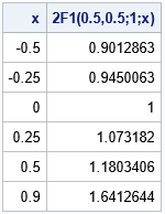
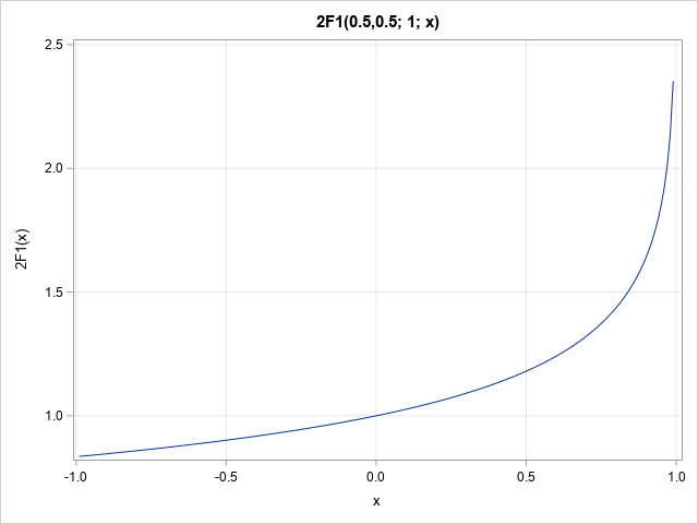
The table shows a few values of Gauss's hypergeometric function for the parameters (a,b;c)=(0.5,0.5;1). You can visualize the function on the open interval (-1, 1) by using the following statements:

x = T( do(-0.99, 0.99, 0.01) );
F = Hypergeometric2F1(x, parm);
 
title "2F1(0.5,0.5; 1; x)";
call series(x, F) grid={x y} label={'x' '2F1(x)'};

Summary

Although I am not an expert on hypergeometric functions, this article shares a few tips for computing Gauss's hypergeometric function, $\,_{2}F_{1}(a,b;c; x)$ in SAS for real arguments and for the special case c > b > 0. For this parameter range, you can compute the hypergeometric function as a definite integral. As shown in the next blog post, you can use this computation to compute the PDF of a certain probability distribution.

You can download the SAS IML functions that evaluate Gauss's hypergeometric function from GitHub.

References

Beukers, F. (2014) "Hypergeometric Functions, How Special Are They?" Notices of the AMS, 61(1), p. 48-56.
Weisstein, Eric W. "Hypergeometric Function." From MathWorld--A Wolfram Web Resource.

Blogs