This article describes how you can evaluate the Lambert W function in SAS/IML software. The Lambert W function is defined implicitly: given a real value x, the function's value w = W(x) is the value of w that satisfies the equation w exp(w) = x. Thus, W is the inverse of the function g(w) = w exp(w).

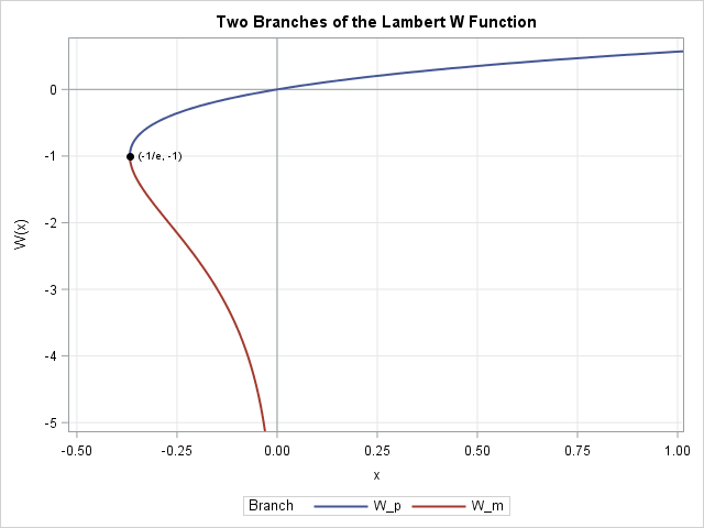
Because the function g has a minimum value at w = –1, there are two branches to the Lambert W function. Both branches are shown in the adjacent graph. The top branch is called the principal (or positive) branch and is denoted W_p. The principal branch has domain x ≥ -1/e and range W(x) ≥ -1. The lower branch, denoted by W_m, is defined on -1/e ≤ x < 0 and has range W(x) ≤ –1. The subscript "m" stands for "minus" since the range contains only negative values. Some authors use W₀ for the upper branch and W_-1 for the lower branch.

Both branches are used in applications, but the lower branch W_m is useful for the statistical programmer because you can use it to simulate data from heavy-tailed distribution. Briefly: for a class of heavy-tailed distributions, you can simulate data by using the inverse CDF method, which requires evaluating the Lambert W function. This is shown in a companion article: "Simulate data from a generalized Gaussian distribution."

Calling the Lambert W function in SAS/IML

SAS IML software supports the LAMBERTW function, which can evaluate either branch of the Lambert W function. The following program evaluates the Lambert W function on each branch:

proc iml;
/* principal branch: Call  LambertW(x, 0) or  use LambertW(x) b/c 0 is default */
x = do(-1/exp(1), 1, 0.01);
Wp = LambertW(x, 0);   /* principal branch */
 
title "Lambert W Function: Principal Branch";
call series(x, Wp) grid={x y} other="refline 0/axis=x; refline 0/axis=y";
 
/* lower branch */
x = do(-1/exp(1), -0.01, 0.001);
Wm = LambertW(x, -1);
title "Lambert W Function: Lower Branch";
call series(x, Wm) grid={x y};

The graphs are not shown because they are the same as the two branches in the graph at the beginning of this article.

Summary

The Lambert W function is included as a built-in function, called LAMBERTW. It is part of SAS/IML software as of SAS/IML 14.3 (SAS 9.4M5). The Lambert W function is the inverse function of g(w) = w exp(w). Although the Lambert W function does not have a closed-form solution, you can implement it numerically to high precision.

If you are running an earlier version of SAS, the SAS/IML language provides an excellent environment for implementing new functions. The Appendix shows how to implement functions that evaluate the upper and lower branches of the Lambert W function. The functions use one or two Halley iterations to quickly converge within machine precision.

Appendix: Defining the Lambert W function prior to SAS/IML 14.3

The Lambert W function was released in SAS/IML 14.3, which was part of SAS 9.4M5. If you are using an earlier versions of SAS/IML, you can download the SAS/IML functions that evaluate each branch of the Lambert W function. Both functions use an analytical approximation for the Lambert W function, followed by one or two iterations of Halley's method to ensure maximum precision. In this implementation:

• The LambertWp function implements the principal branch W_p. The algorithm constructs a direct global approximation on [-1/e, ∞) based on Boyd (1998).
• The LambertWm function implements the second branch W_m. The algorithm follows Chapeau-Blondeau and Monir (2002) (hereafter CBM). The CBM algorithm approximates W_m(x) on three different domains. The approximation uses a series expansion on [-1/e, -0.333), a rational-function approximation on [-0.333, -0.033], and an asymptotic series expansion on (-0.033, 0).

%include "C:\MyPath\LambertW.sas";      /* specify path to file */
proc iml;
load module=(LambertWp LambertWm);
 
x = do(-1/exp(1), 1, 0.01);
Wp = LambertWp(x);   /* Wp = LambertW(x, 0);    <== SAS/IML 14.3 and later */
title "Lambert W Function: Principal Branch";
call series(x, Wp) grid={x y} other="refline 0/axis=x; refline 0/axis=y";
 
x = do(-1/exp(1), -0.01, 0.001);
Wm = LambertWm(x);   /* Wm = LambertW(x, -1);   <== SAS/IML 14.3 and later */
title "Lambert W Function: Lower Branch";
call series(x, Wm) grid={x y};

The graphs are not shown because they are indistinguishable from the graph at the beginning of article.

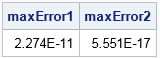
You can use a simple error analysis to investigate the accuracy of the pre-14.3 functions. After computing w = W(x), apply the inverse function g(w) = w exp(w) and see how close the result is to the input values. The LambertWp and LambertWm functions support an optional second parameter that specifies how many Halley iterations are performed. For LambertWm, only one iteration is performed by default. You can specify "2" as the second parameter to get two Halley iterations. The following statements show that the maximum error for the default computation is 2E-11 on (-1/e, -0.01). The error decreases to 5E-17 if you request two Halley iterations.

x = do(-1/exp(1), -0.01, 0.001);
Wm = LambertWm(x);            /* default precision: 1 Halley iteration */
g = Wm # exp(Wm);             /* apply inverse function */
maxError1 = max(abs(x - g));  /* maximum error */
 
Wm = LambertWm(x, 2);         /* higher precision: 2 Halley iterations */
g = Wm # exp(Wm);
maxError2 = max(abs(x - g));
print maxError1 maxError2;