Although statisticians often assume normally distributed errors, there are important processes for which the error distribution has a heavy tail. A well-known heavy-tailed distribution is the t distribution, but the t distribution is unsuitable for some applications because it does not have finite moments (means, variance,...) for small parameter values. An alternative choice for a heavy-tailed distribution is the generalized Gaussian distribution, which is the topic of this article.

The generalized Gaussian distribution

The generalized Gaussian distribution has a standardized probability density of the form f(x) = B exp( -|Ax|^α ), where A(α) and B(α) are known functions of the exponent parameter α > 0. When 0 < α < 2, the generalized Gaussian distribution (GGD) is a heavy-tailed distribution that has finite moments. The distribution has applications in finance and signal processing.

The following SAS statements evaluate the GGD density function for four values of the shape parameter α. The SGPLOT procedure graphs the density functions (adapted from Nardon and Pianca (2009)):

data GenGauss;
mu=0; sigma=1;  /* location=mu and scale=sigma */
do alpha = 0.5, 1, 2, 5;
   A = sqrt( Gamma(3/alpha) / Gamma(1/alpha) ) / sigma;   /* A(alpha, sigma) */
   B = (alpha/2) / Gamma(1/alpha) * A;                    /* B(alpha, sigma) = normalizing constant */
   do x = -3 to 3 by 0.05;
      pdf = B*exp(-(A*abs(x-mu))**alpha);
      output;
   end;
end;
run;
 
title "Generalized Gaussian Densities";
title2 "(*ESC*){unicode mu}=0; (*ESC*){unicode sigma}=1"; 
proc sgplot data=GenGauss;
   series x=x y=pdf / group=alpha;
   yaxis grid label="Density of Generalized Gaussian";
   keylegend / across=1 opaque location=inside position=right;
run;

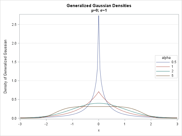
The density for α=1/2 is sharply peaked and has heavy tails. The distribution for α=1 is the Laplace distribution, which also has a sharp peak at the mean. The distribution for α=2 is the standard normal distribution. For α=5, the distribution is platykurtic: it has a broad flat central region and thin tails.

This article uses only the standardized distribution that has zero mean and unit variance. However, the functions are all written to support a location parameter μ and a scale parameter σ.

Simulate random values from the generalized Gaussian distribution

Nardon and Pianca (2009) describe an algorithm for simulating random variates from the generalized Gaussian distribution: simulate from a gamma distribution, raise that variate to a power, and then randomly multiply by ±1. You can implement the simulation in the SAS DATA step or in the SAS/IML language. The following SAS/IML program defines a function for generating random GGD values:

proc iml;
start Rand_GenGauss(N, mu=0, sigma=1, alpha=0.5);
   n1 =N[1]; n2 = 1;                         /* default dimensions for returned matrix */
   if nrow(N)>1 | ncol(N)>1 then n2 = N[2];  /* support n1 x n2 matrices */
   x = j(n1,n2);  sgn = j(n1,n2);
   /* simulate for mu=0 and sigma=1, then scale and translate */
   A = sqrt( Gamma(3/alpha) / Gamma(1/alpha) );
   b = A##alpha;
   call randgen(x, "Gamma", 1/alpha, 1/b);   /* X ~ Gamma(1/alpha, 1/b) */
   call randgen(sgn, "Bernoulli", 0.5); 
   sgn = -1 + 2*sgn;                         /* random {-1, 1} */
   return mu + sigma * sgn # x##(1/alpha);
finish;
 
/* try it out: simulate 10,000  random variates */
call randseed(12345);
x = Rand_GenGauss(10000, 0, 1, 1/2);         /* X ~ GGD(mu=0, sigma=1, alpha=1/2) */
 
title "Generalized Gaussian Distribution";
title2 "mu=0, sigma=1, alpha=1/2";
call histogram(x);

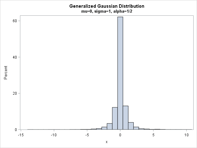
For α=1/2, most of the simulated values are near 0, which is the mean and mode. The bulk of the remaining values are in the interval [-5,5]. However, a very small percentage (about 0.5%) are more extreme than these values. For this sample, the range of the simulated data is about [-14 , 11], so you can see that this distribution is useful for simulations in which the magnitude of errors can be more extreme than normal errors.

The generalized Gaussian distribution with exponent 1/2

The cumulative distribution function for the generalized Gaussian distribution does not have a closed-form solution in terms of elementary functions. However, there are a few values of α for which the equations simplify, including α=1/2. Chapeau-Blondeau and Monir (2002) note that the generalized Gaussian distribution with α=1/2 is especially useful in practice because its quantile function (inverse CDF) can be explicitly expressed in terms of the Lambert W function.

The CDF for the GGD with α=1/2 can be computed separately for x ≤ 0 and for x > 0, as shown below:

/* CDF for generalized Gaussian distribution with alpha=1/2 */
start CDF_GenGaussHalf(x);
   y = sqrt(abs(2*sqrt(30)*x));
   cdf = 0.5*(1+y)#exp(-y);     /* CDF for x <= 0 */
   idx = loc(x>0);              /* if x > 0, reflect: CDF(x) = 1 - CDF(-x) */
   if ncol(idx)>0 then do;
      cdf[idx] = 1 - cdf[idx];
   end;
   return cdf;
finish;
 
p = CDF_GenGaussHalf(-5);    /* P(X< -5) for X ~ GDD(0,1, alpha=1/2) */
print p;                     /* 0.0025654 */

You can use the CDF function to evaluate the probability that a random GGD observation is less than -5. The answer is 0.0026. By symmetry, the probability that a random variate is outside of [-5,5] is 0.0052, which agrees with the empirical proportion in the random sample in the previous section.

The inverse CDF for the GGD with α=1/2 can be implemented by calling the Lambert W function. (Technically, the lower branch of the Lambert W function.) You can download functions that implement the Lambert W function in SAS/IML. The following SAS/IML statements assume that you have downloaded the Lambert W functions and stored the modules, so that they are available by using the LOAD statement. Just as the CDF was defined in two parts, the inverse CDF is defined in two parts. [UPDATE: The LambertW function is now available as a built-in function in SAS/IML; use it instead of the LambertWm function.]

/* Use Lambert W function to compute the quantile function
   (inverse CDF) for generalized Gaussian distribution with alpha=1/2 */
load module=(LambertWm);          /* load function for the Lambert W function */
start Quantile_GenGaussHalf(x);
   q = j(nrow(x), ncol(x), 0);
   idx = loc(x<0.5);              /* invert CDF for x < 0.5 */
   if ncol(idx)>0 then do;
      y = -2 * x[idx] / exp(1);
      q[idx] = -1/(2*sqrt(30)) * (1 + LambertWm(y))##2;
   end;
   if ncol(idx)=nrow(x)*ncol(x) then return q;  /* all found */
 
   idx = loc(x=0.5);              /* quantile for x=0.5 */
   if ncol(idx)>0 then q[idx] =  0;
   idx = loc(x>0.5);              /* invert CDF for x > 0.5 */
   if ncol(idx)>0 then do;
      y = -2 * (1-x[idx]) / exp(1);
      q[idx] =  1/(2*sqrt(30)) * (1 + LambertWm(y))##2;
   end;
   return q;
finish;
 
q = Quantile_GenGaussHalf(0.975);  /* find q such that P(X < q) = 0.975 */
print q;                           /* 2.0543476 */

The output (not shown) is q = 2.05, which means that the interval [-2.05, 2.05] contains 95% of the probability for the standardized GGD when α=1/2. Compare this interval with the familiar interval [-1.96, 1.96], which contains 95% of the probability for the standard normal distribution.

References

To learn more about the generalized Gaussian distribution, with an emphasis on parameter value α=1/2, see the following wwll-written papers, which expand the discussion in this blog post:

• F. Chapeau-Blondeau and A. Monir (2002), "Numerical Evaluation of the Lambert W Function and Application to Generation of Generalized Gaussian Noise With Exponent 1/2," IEEE Trans. on Sig. Processing.
• Nardon and Pianca (2009; download preprint 2006). "Simulation techniques for generalized Gaussian densities," J. Stat. Comp. and Sim.