Continued fractions show up in surprising places. They are used in the numerical approximations of certain functions, including the evaluation of the normal cumulative distribution function (normal CDF) for large values of x (El-bolkiny, 1995, p. 75-77) and in approximating the Lambert W function, which has applications in the modeling of heavy-tailed error processes. This article shows how to use SAS to convert a rational number into a finite continued fraction expansion and vice versa.

What is a continued fraction?

I discussed continued fractions in a previous post about the continued fraction expansion of pi. Recall that every real number x can be represented as a continued fraction:

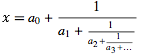
In this continued fraction, a₀ is the integer portion of the number and the a_i for i > 0 are positive integers that represent the noninteger portion. Because all the fractions have 1 in the numerator, the continued fraction can be compactly represented by specifying only the integers: x = [a₀; a₁, a₂, a₃, ...]. Every rational number is represented by a finite sequence; every irrational number requires an infinite sequence. Notice that the decimal representation of a number does NOT have this nice property: 1/3 is rational but its decimal representation is infinite.

Convert a finite continued fraction to a rational number

My article about the continued fraction expansion of pi contains a few lines of SAS code that compute the decimal representation of a finite continued fraction. Since every finite continued fraction corresponds to a rational number, you can modify the algorithm to compute the rational number instead of a decimal approximation.

The algorithm is straightforward. Given a vector
a = [a₀; a₁, a₂, ..., a_k],
start at the right side, form the fraction s_k = 1 / a_k. Then move to the left and compute the fraction s_k-1 = a_k-1 + s_k. Continue moving to the left until all fractions are added. In the SAS/IML language (or in the SAS DATA step), you can represent each fraction as a two-element vector where the first element is the numerator of the fraction and the second is the denominator of the fraction. This leads to the following algorithm that computes a rational number from a finite continued fraction expansion:

proc iml;
start ContinuedFrac(_a);
   a = colvec(_a);
   f = a[nrow(a)] // 1;         /* trick: start with reciprocal */
   do i = nrow(a)-1 to 1 by -1; /* evaluate from right to left */
      f = f[2:1];               /* take reciprocal */
      f[1] = a[i]*f[2] + f[1];  /* compute new numerator */
   end;
   return f;
finish;
 
a = {3, 4, 12, 4}; 
f = ContinuedFrac(a);      /* 649 / 200 */
pi = {3, 7,15,1,292,1,1,1,2,1,3,1};
f_pi = ContinuedFrac(pi);  /* 5419351 / 1725033 */
e = {2, 1,2,1,1,4,1,1,6,1,1,8};
f_e = ContinuedFrac(e);    /* 23225 / 8544 */
print (f||f_pi||f_e)[r={"Numer" "Denom"} c={"f" "f_pi" "f_e"}];

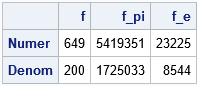
The examples show a few continued fraction expansions and the rational numbers that they represent:

• The continued fraction expansion (cfe) [3; 4, 12, 4] corresponds to the fraction 649 / 200.
• The 12-term partial cfe for pi corresponds to the fraction 5419351 / 1725033. You might have learned in grade school that 22/7 is an approximation to pi. So, too, is this fraction.
• The partial cfe for e (using 12 terms) corresponds to the fraction 23225 / 8544.

Rational numbers to continued fractions

You can program the inverse algorithm to produce the cfe from a rational number. The algorithm is called the Euclidean algorithm and consists of finding the integer part, subtracting the integer part from the original fraction to obtain a remainder (expressed as a fraction), and then repeating this process. The process terminates for every rational number. In the SAS/IML language, the Euclidean algorithm looks like this:

start EuclidAlgRational(val, nSteps=10);
   a = j(nSteps, 1, .);
   x = val;
   done = 0;
   do i = 1 to nSteps while(^done);
      a[i] = floor(x[1] / x[2]);
      x[1] = x[1] - a[i]*x[2];  /* remainder */
      if x[1]=0 then done=1;
      x = x[2:1];               /* reciprocal */
   end;
   idx = loc(a=.);
   if ncol(idx)>0 then a = colvec(remove(a, idx));
   return a;
finish;
 
v = {649, 200};          /* = [3,4,12,4] */
a = EuclidAlgRational(v);
v = {5419351, 1725033};  /* pi = [3; 7,15,1,292,1,1,1,2,1,3,1,...] */
a_pi = EuclidAlgRational(v);
v = {23225, 8544};       /* e = [2; 1,2,1,1,4,1,1,6,1,1,8,...] */
a_e = EuclidAlgRational(v);
print a a_pi a_e;

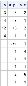
Each column of the table shows the continued fraction representations of a rational number. The output shows that the ContinuedFrac and EuclidAlgRational functions are inverse operations: each function undoes the action of the other.

Two amazing properties of the continued fraction representation

There are some very interesting mathematical properties of continued fractions. Two statistical properties are discussed in Barrow (2000), "Chaos in Numberland: The secret life of continued fractions." Both properties are illustrated by the first 97 terms in the continued fraction expansion of pi, which are
π = [3; 7, 15, 1, 292, 1, 1, 1, 2, 1, 3, 1, 14, 2, 1, 1, 2, 2, 2, 2, 1, 84, 2, 1, 1,
15, 3, 13, 1, 4, 2, 6, 6, 99, 1, 2, 2, 6, 3, 5, 1, 1, 6, 8, 1, 7, 1, 2, 3, 7,
1, 2, 1, 1, 12, 1, 1, 1, 3, 1, 1, 8, 1, 1, 2, 1, 6, 1, 1, 5, 2, 2, 3, 1, 2,
4, 4, 16, 1, 161, 45, 1, 22, 1, 2, 2, 1, 4, 1, 2, 24, 1, 2, 1, 3, 1, 2, 1, ...]

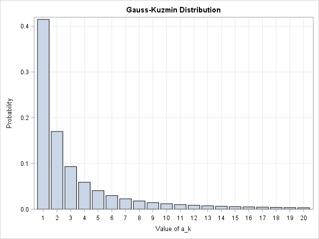
The first property concerns the probability distribution of the a_k for sufficiently large values of k. Notice that the continued fractions in this article mostly contain small integers such as 1, 2, 3, and 4. It turns out that this is generally true. For almost every irrational number in (0,1) and for k sufficiently large, the k_th term a_k is more likely to be a small integer than a large integer. In fact, the Gauss-Kuzmin theorem states that the distribution of a_k (thought of as a random variable) asymptotically approaches the probability mass function P(a_k = t) = -log₂(1 - 1/(1+t)²), which is shown below for t ≤ 20. Thus, for a random irrational number, although the value of, say, the 1000th term in the continued fraction expansion could be any positive integer, it is probably less than 20!

The second interesting mathematical property is Khinchin's Theorem, which states that for almost every irrational number in (0,1), the geometric mean of the first t digits in the continued fraction expansion converges (as t → ∞) to a constant called Khinchin's constant, which has the value 2.685452001.... For example, the first 97 terms in the continued fraction expansion of pi have a geometric mean of 2.685252.