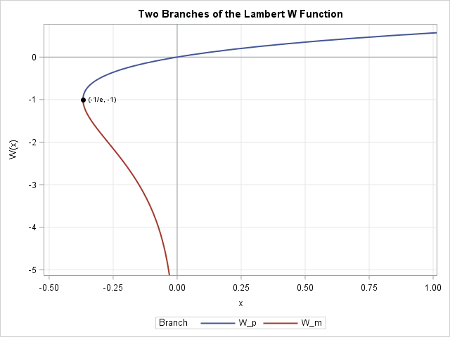
I previously wrote an article about the Lambert W function. The Lambert W function is the inverse of the function g(x) = x exp(x). This means that you can use it to find the value of x such that g(x)=c for any value of c in the range of g, which is the interval (0, ∞). Equations like this are called implicit equations: The right-hand side (c) is a parameter, and you want to find a value (or values) in the domain of g that satisfies the equation. In terms of the Lambert W function, the solution is given explicitly as x = W(c). The graph of the Lambert W function is shown to the right.
The LAMBERTW function is included in SAS IML software. This article shows a few examples of using SAS and the Lambert W function to solve implicit equations in which the variable (x) occurs as an exponent and also in a linear term. For each equation, you can convert it into a standard form and apply the Lambert W function. For example, this article shows how to use the Lambert W function to solve the following equations for x:
- x exp(x) = c. This is the canonical Lambert equations. The value c is a parameter.
- x bx = c. This generalizes the Lambert equation. Instead of a base of e, any base (b) is permitted.
- exp(x) = m*x + b. This does not look like the Lambert equation, but it can be manipulated into the standard Lambert form. In this equation, there is an exponential function on one side and a linear function on the other. Equivalently, you can express this equation in the form exp(-cx) = a(x – r) for different constants.
Inverses for functions that are not one-to-one
Recall that a function is one-to-one if each element of the domain is mapped to a unique element of the range. Inverse functions can be difficult to work with when the underlying function is not one-to-one. Compare two of the most famous inverse functions: LOG and SQRT.
- The EXP function, x → exp(x), is one-to-one. Given any value of c in the range of EXP, there is a unique value of x such that exp(x) = c. We define the LOG function to be the inverse of the exponential function and write the solution explicitly as x = log(c). Of course, c must be in the range of the EXP function (which is c > 0) or else the equation has no real solution.
- The squaring function, x → x2, is not one-to-one. Given a value of c > 0, there are two values of x such that x2 = c. Thus, there isn't a unique inverse function. Nevertheless, we can define the function SQRT as the "principal branch" of the inverse function and, by symmetry, use -SQRT as a second branch. Consequently, we can write the two solutions of x2 = c as {±sqrt(c)} when c ≥ 0.
The Lambert function is the inverse of g(x) = x exp(x). For c ≥ 0, there is a unique value of x that solves x exp(x) = c. However, when -1/e < c < 0, the equation has two solutions, one where x > -1 and the other where x < -1. We use the symbol W0 for the principal or "upper" branch of the inverse function that returns x ≥ -1. The "lower" branch, denoted by W-1, returns x ≤ -1.
Example 1: Use the Lambert function in SAS

Let's first solve the classical Lambert equation x exp(x) = c for the parameter c=1. The graph of the function is shown to the right, along with a horizontal line for c = 1.
The Lambert function is the inverse function. Therefore, by definition, the solution is x = W(c). In other words, the curve intersects the upper horizontal line at x1 = W(1). Since c > 0, the solution lies solely on the upper branch, x1 = W0(1).
You can obtain a numerical solution by using the LAMBERTW function in SAS IML:
proc iml; c1 = 1; xSoln = LambertW(c1); print c1 xSoln; |

The solution is x = 0.5671.
Now let's solve the equation x exp(x) = c for the parameter c= -0.3. Because -1/e < c < 0, the curve intersects the horizontal line at c in two places. One solution is x1 = W-1(-0.3) and the other is x2 = W0(-0.3). To make it easier to return all solutions, you can write an IML function that tests the value of c and returns zero, one, or two solutions, as appropriate:
/* Function to evaluate all branches of the Lambert W function. The expression W(z) - has one solution when z >= 0 - has two solutions when -1/e <= z < 0 - has zero solutions when z < -1/e */ start W_both(z); if z >= 0 then return LambertW(z); else if -exp(-1) <= z then return LambertW(z,-1) // LambertW(z,0); else return .; finish; store module=(W_both); /* store the function for later use */ c2 = -0.3; xSoln = W_both(c2); print c2 xSoln; |

The two solutions are x1 = -1.7813 and x2 = 0.4894.
Example 2: A different base
The classical Lambert equation is x ex = c, where e ≈ 2.71828... is the base of the natural logarithm.
It is not too surprising that you can also use the Lambert W function to
solve an equation of the form
\(x b^x = c\)
where b > 0 is a different base, such as b=2 or b=3. If b=1, the equation is trivial, so assume b ≠ 1.
When b > 1, the graph of this equation looks similar to the graph shown in the previous section.
It is not difficult to manipulate the equation into the Lambert form.
Recall that \(b = e^{\ln b}\) for any b > 0, which means that \(x b^x = x e^{x \ln b}\).
We can multiply both sides of the equation by \(\ln b\) to obtain:
\(x \ln(b) b^x = x \ln(b) e^{x \ln(b)} = c \ln(b)\)
By making the substitution \(u = x \ln(b)\), we obtain the standard
Lambert equation \(u e^u = c \ln(b)\), so the solution is \(u = W(c \ln(b))\) or \(x = W(c \ln(b)) / \ln(b)\).
You can use PROC IML to obtain the solution to x bx = c, where b=3 and c= -0.3, as follows:
/* solve x*3^x = -0.3 */ b = 3; c = -0.3; z = c*log(b); xSoln = W_both(z) / log(b); print b c xSoln; |

Example 3: A linear term

The Wikipedia article on the Lambert W function states that
the Lambert W function "expresses exact solutions to transcendental algebraic equations (in x) of the form
\(e^{-cx} = a(x-r)\)
where a, c and r are real constants." The solution is derived in the Appendix. The solution is
\(x = r+ W\left({\frac{c\,e^{-cr}}{a}}\right) / c\)
In contrast to the standard Lambert equation, in this equation the exponential term and the linear term are on the opposite sides of the equal sign. That means that you are looking for the intersection of an exponential curve and a diagonal line. The plot to the right shows the graphs of the left-hand and right-hand sides of the equation for a=0.5, r = -2.5, and c = -1. The graphs intersect in two points, which can be found by using the Lambert W function:
/* solve a*(x - r) = exp(-cx) for x */ a = 0.5; r = -2.5; c = -1; z = c * exp(-c*r) / a; xSoln = r + W_both(z) / c; print a r c xSoln; |

If you have an equation of the form exp(x) = m*x + b, you can transform it to the form that I solved. I leave the transformation as an exercise.
Summary
The Lambert W function solves the implicit equation x exp(x) = c for x. Depending on the value of c, the equation has either 0, 1, or 2 real solutions. There are a number of equations that can be transformed into the standard form and be solved by the Lambert W function. In addition to the standard form, this article shows how to use SAS and the Lambert W function to solve equations of the form
- x bx = c
- exp(-cx ) = a(x-r)
You can use the Lambert W function in many applications. For example, you can use use the Lambert W function to compute the quantiles of the generalized Gaussian distribution. The paper by Corless et al. (1996, Advances in Computational Mathematics) provides many more examples of applications of the Lambert W function. It is an easy paper to read if you want to appreciate the power of the Lambert W function.
Appendix: Derivation of a Lambert equation solution
The Wikipedia article on the Lambert W function states that
the solution of the equation
\(e^{-cx} = a(x-r)\)
where a, c and r are real constants is obtained by using the Lambert W function:
\(x = r+ W\left({\frac{c\,e^{-cr}}{a}}\right) / c\)
Here is how to derive that solution.
Starting with the given equation, put all the terms that contain x on one side of the equation:
\(\frac{1}{a} = (x-r) \exp(c x)\)
To get the right-hand side in standard form, the quantity multiplying the exponential term must be the same as the quantity in the exponent.
Thus, multiply both sides by \(c \exp(-cr )\) to obtain:
\(c \exp(-cr) / a = c(x-r) \exp(c(x-r))\)
From here, the solution is straightforward. Perform the substitution \(u = c(x-r)\) to put the equation in standard form. The
solution to the transformed equation is
\(u = W\left( c \exp(-c r)/ a) \right)
\)
and it follows that
\(x = r + W\left( c \exp(-c r)/ a) \right) / c
\)

1 Comment
Pingback: Pi to the power of pi - The DO Loop