Least-squares optimization and the Gauss-Newton method

A previous article showed how to use SAS to compute finite-difference derivatives of smooth vector-valued multivariate functions. The article uses the NLPFDD subroutine in SAS/IML to compute the finite-difference derivatives. The article states that the third output argument of the NLPFDD subroutine "contains the matrix product J`*J, where J is the Jacobian matrix. This product is used in some numerical methods, such as the Gauss-Newton algorithm, to minimize the value of a vector-valued function."

This article expands on that statement and shows that you can use the SAS/IML matrix language to implement the Gauss-Newton method by writing only a few lines of code.

The NLPFDD subroutine has been in SAS/IML software since SAS version 6. In SAS Viya, you can use the FDDSOLVE subroutine, which is a newer finite-difference function that has a syntax similar to the NLPFDD subroutine.

A review of least-squares minimization

Statisticians often use least-squares minimization in the context of linear or nonlinear least-squares (LS) regression. In LS regression, you have an observed set of response values {Y1, Y2, ..., Yn}, and you fit a parametric model to obtain a set of predicted values {P1, P2, ..., Pn}. These predictions depend on parameters, and you try to find the parameters that minimize the sum of the squared residuals, || P_i - Y_i ||² for i=1, 2, ..., n.

In this formula, the parameters are not explicitly written, but this formulation is the least-squares minimization of a function that maps each parameter to the sum of squared residuals. Abstractly, if F: Rⁿ → R^m is a smooth vector-valued function with m components, then you can write it as F(x) = (F₁(x), F₂(x), ..., F_m(x)). In most applications, the dimension of the domain is less than the dimension of the range: n < m. The goal of least-square minimization is to find a value of x that minimizes the sum of the squared components of F(x). In vector form, we search for a value of x that (locally) minimizes || F(x) ||². Equivalently, the problem is often formulated so that you minimize (1/2) || F(x) ||². The factor of 1/2 simplifies the expression for the derivative of the objective function.

Visualize a least-squares function

The previous article used the following vector-valued function:

proc iml;
 
q = {0, 2, 1};               /* define a point in R^3 */
start VecF(st) global(q);    /* compute vector from q to a point on a cylinder */
   s = st[1]; t = st[2];
   F = j(3, 1, .);
   F[1] = cos(s) - q[1];
   F[2] = sin(s) - q[2];
   F[3] =     t  - q[3];
   return( F );
finish;

Geometrically, this function represents the vector from q = (0, 2, 1) to a point on a cylinder in R³. Therefore, the vector-valued function is minimized when (s,t) = (pi/2, 1), since that is the point on the cylinder closest to the point q, which is not on the cylinder.

Let's visualize the function (1/2) || F(s,t) ||² for (s,t) values near (pi/2. 1). You can use the EXPANDGRID function to create a uniform grid of points in the (s,t) domain. For each point on the grid, you can use the following statements to compute (one-half) the sum of the squares of the vector-valued function. To compute the sum of squared components, you can use the SSQ function or the NORM function, but I have decided to use the inner-product F`*F.

/* create heat map of VecF */
s = do(1, 2.1, 0.02);       /* horiz grid points */
t = do(0.5, 1.5, 0.02);     /* vert grid points */
st = expandgrid(s, t);
z = j(nrow(st), 1);
do i = 1 to nrow(st);
   F = VecF( st[i,] ); 
   z[i] = 0.5 * F`*F;       /* 1/2 sum of squares of components */
end;
 
result = st||z;
create Heat from result[c={'s' 't' 'z'}]; append from result; close;
 
submit;
title "1/2 || F(x,y) ||^2";
proc sgplot data=Heat;
   heatmapparm x=s y=t colorresponse=z / colormodel=ThreeColorRamp;
   refline 1.571/axis=x label='pi/2' labelpos=min; refline 1/axis=y;
run;
endsubmit;

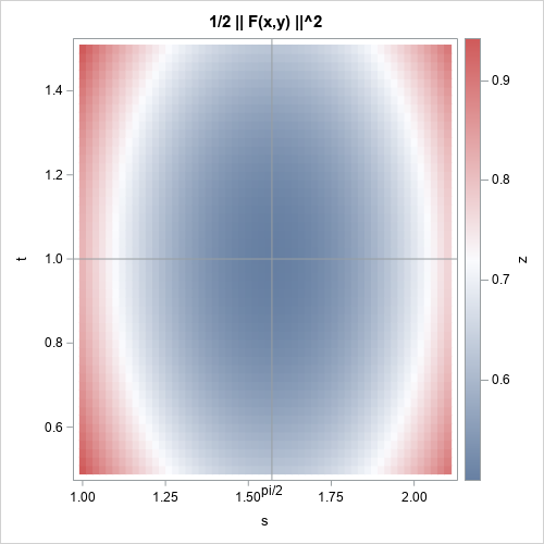
The graph shows the values of z = (1/2) ||F(s,t)||² on a uniform grid. The reference lines intersect at (pi/2, 1), which is the minimum value of z.

The Gauss-Newton method for minimizing least-squares problems

One way to solve a least-squares minimization is to expand the expression (1/2) ||F(s,t)||² in terms of the component functions. You get a scalar function of (s,t), so you can use a traditional optimization method, such as the Newton-Raphson method, which you can call by using the NLPNRA subroutine in SAS/IML. Alternatively, you can use the NLPLM subroutine to minimize the least-squares problem directly by using the vector-valued function. In this section, I show a third method: using matrix operations in SAS/IML to implement a basic Gauss-Newton method from first principles.

The Gauss-Newton method is an iterative method that does not require using any second derivatives. It begins with an initial guess, then modifies the guess by using information in the Jacobian matrix. Since each row in the Jacobian matrix is a gradient of a component function, the Gauss-Newton method is similar to a gradient descent method for a scalar-valued function. It tries to move "downhill" towards a local minimum.

Rather than derive the formula from first principles, I will merely present the Gauss-Newton algorithm, which you can find in Wikipedia and in course notes for numerical analysis (Cornell, 2017):

Make an initial guess for the minimizer, x0. Let x = x0 be the current guess.
Evaluate the vector F ≡ F(x) and the Jacobian J ≡ [ ∂F_i / ∂x_j ] for i=1,2,..,m and j=1,2...,n. The NLPFDD subroutine in SAS/IML enables you to evaluate the function and approximate the Jacobian matrix with a single call.
Find a direction that decreases || F(x) || by solving the linear system (J`J) h = -J`*F for h.
Take a step in the direction of h and update the guess: x_new = x + α h for some α in (0, 1).
Go to Step 2 until the problem converges.

For any point x in the domain of F, the NLPFDD subroutine returns three results: F, J, and the matrix product J`*J. These are exactly the quantities that are needed to perform the Gauss-Newton method! The following statements implement the algorithm for an initial guess x0 = (2, 0.5):

/* Gauss-Newton line-search method for minimizing || VecF(x) || */
x0 = {2  0.5};       /* initial guess for (s,t) */
parm = {3, 00, .};   /* function has 3 components, use forward difference */
nSteps = 10;         /* take 10 steps regardless of convergence */
alpha = 0.6;         /* step size for line search */
 
path = j(nSteps+1, 2);  /* save and plot the approximations */
path[1,] = x0;
/* start the Gauss-Newton method */
x = x0;
do i = 1 to nSteps;
   call nlpfdd(F, J, JtJ, "VecF", x) par=parm; /* get F, J, and J`J at x */
   h = solve(JtJ, -J`*F);   /* h points downhill */
   x = x + alpha*h`;        /* update the current guess */
   path[i+1,] = x;          /* remember this point */
end;
 
/* write the iterates to a data set */
create path from path[c={'px' 'py'}]; append from path; close;
 
submit alpha;
data All; set Heat path; run;
 
title "Path of Gauss-Newton Minimization";
title2 "alpha = &alpha";
proc sgplot data=All noautolegend;
   heatmapparm x=s y=t colorresponse=z / colormodel=ThreeColorRamp;
   refline 1.571/axis=x label='pi/2' labelpos=min; refline 1/axis=y;
   series x=px y=py / markers;
run;
endsubmit;

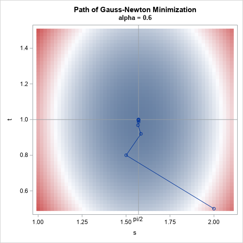
The graph overlays the path of the Gauss-Newton approximations on the heat map of (1/2) || F(s,t) ||². For each iterate, you can see that the search direction appears to be "downhill." A more sophisticated algorithm would monitor the norm of h to determine when to step. You can also use different values of the step length, α, or even vary the step length as you approach the minimum. I leave those interesting variations as an exercise.

The main point I want to emphasize is that the NLPFDD subroutine returns all the information you need to implement the Gauss-Newton method. Several times, I have been asked why the NLPFDD subroutine returns the matrix J`*J, which seems like a strange quantity. Now you know that J`*J is one of the terms in the Gauss-Newton method and other similar least-squares optimization methods.

Verify the Gauss-Newton Solution

As I mentioned earlier, SAS/IML software supports two subroutines for solving least-squares minimization problems. The NLPHQN subroutine is a hybrid quasi-Newton algorithm that is similar to (but more sophisticated than) the Gauss-Newton method. Let's use the NLPHQN subroutine to solve the same problem and compare the solutions:

/* solve same problem by using NLPHQN (hybrid quasi-Newton method) */
optn = {3 1};     /* tell NLPQN that VecF has three components; print some partial results */
call NLPHQN(rc, xSoln, "VecF", x0) OPT=optn; 
print (path[11,])[c={'s' 't'} L="Soln from Gauss-Newton"],
       xSoln[c={'s' 't'} L="Soln from NLPHQN"];

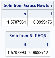
The solution from the hybrid quasi-Newton method is very close the Gauss-Newton solution. If your goal is to solve a least-squares minimization, use the NLPHQN (or NLPLM) subroutine. But you might want to implement your own minimization method for special problems or for educational purposes.

Summary

In summary, this article shows three things:

For a vector-valued function, the NLPFDD subroutine evaluates the function and uses finite-difference derivatives to approximate the Jacobian (J) at a point in the domain. The subroutine also returns the matrix product J`*J.
The three quantities from the NLPFDD subroutine are exactly the three quantities needed to implement the Gauss-Newton method. By using the NLPFDD subroutine and the matrix language, you can implement the Gauss-Newton method in a few lines of code.
The answer from the Gauss-Newton method is very similar to the answer from calling a built-in least-squares solver, such as the NLPHQN subroutine.

Blogs