I previously showed how to use SAS to compute finite-difference derivatives for smooth scalar-valued functions of several variables. You can use the NLPFDD subroutine in SAS/IML software to approximate the gradient vector (first derivatives) and the Hessian matrix (second derivatives). The computation uses finite-difference derivatives to approximate the derivatives.

The NLPFDD subroutine also supports approximating the first derivatives a smooth vector-valued function. If F: Rⁿ → R^m is a vector-valued function with m components, then you can write it as F(x) = (F₁(x), F₂(x), ..., F_m(x)). The Jacobian matrix, J, is the matrix whose (i,j)th entry is J[i,j] = ∂F_i / ∂x_j. That is, the i_th row is the gradient of the i_th component function, F_i, i=1,2,..,m and j=1,2...,n. The NLPFDD subroutine enables you to approximate the Jacobian matrix at any point in the domain of F.

An example of a vector-valued function

A simple example of a vector-valued function is the parameterization of a cylinder, which is a mapping from R² → R³ given by the function
C(s,t) = (cos(s), sin(s), t)
For any specified values of (s,t), the vector C(s,t) is the vector from the origin to a point on the cylinder. It is sometimes useful to consider basing the vectors at a point q, in which case the function F(s,t) = C(s,t) - q is the vector from q to a point on the cylinder. You can define this function in SAS/IML by using the following statements. You can then use the NLPFDD subroutine to compute the Jacobian matrix of the function at any value of (s,t), as follows:

/* Example of a vector-valued function f: R^n -> R^m for n=2 and m=3.
   Map from (s,t) in [0, 2*pi) x R to the cylinder in R^3.
   The vector is from q = (0, 2, 1) to C(s,t)  */
proc iml;
 
q = {0, 2, 1};               /* define a point in R^3 */
/* vector from q to a point on a cylinder */
start VecF(st) global(q);
   s = st[1]; t = st[2];
   F = j(3, 1, .);
   F[1] = cos(s) - q[1];
   F[2] = sin(s) - q[2];
   F[3] =     t  - q[3];
   return( F );
finish;
 
/* || VecF || has local min at (s,t) = (pi/2, 1), so let's evaluate derivatives at (pi/2, 1) */
pi = constant('pi');
x =  pi/2 || 1;              /* value of (s,t) at which to evaluate derivatives */
/* Parameters: the function has 3 components, use forward difference, choose step according to scale of F */
parm = {3, 00, .};           
call nlpfdd(f, J, JtJ, "VecF", x) par=parm;  /* return f(x), J=DF(x), and J`*J */
 
print f[r={'F_1' 'F_2' 'F_3'} L='F(pi/2, 1)'], 
      J[r={'F_1' 'F_2' 'F_3'} c={'d/ds' 'd/dt'} L='DF(pi/2, 1) [Fwd Diff]'];

The program evaluates the function and the Jacobian at the point (s,t)=(π/2, 1). You must use the PAR= keyword when the function is vector-valued. The PAR= argument is a three-element vector that contains the following information. If you specify a missing value, the default value is used.

• The first element is the number of components (m) for the function. By default, the NLPFDD subroutine expects a scalar-valued function (m=1), so you must specify PARM[1]=3 for this problem.
• The second element is the finite-difference method. The function supports several schemes, but I always use either 0 (forward difference) or 1 (central difference). By default, PARM[2]=0.
• The third element provides a way to choose the step size for the finite-difference method. I recommend that you use the default value.

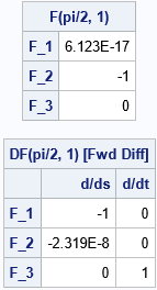
The output shows that the value of the function at (s,t)=(π/2, 1) is {0, -1, 0}. The Jacobian at that point is shown. The gradient of the i_th component function (F_i) is contained in the i_th row of the Jacobian matrix.

• The gradient of the first component function at (π/2, 1) is {-1 0}.
• The gradient of the second component function at (π/2, 1) is {0 0}, which means that F₂ is at a local extremum. (In this case, F₂ is at a minimum).
• The gradient of the third component function is {0 1}.

The NLPFDD subroutine also returns a third result, which is named JtJ in the program. It contains the matrix product J`*J, where J is the Jacobian matrix. This product is used in some numerical methods, such as the Gauss-Newton algorithm, to minimize the value of a vector-valued function. Unless you are writing your own algorithm to perform a least-squares minimization, you probably won't need the third output argument.

Summary

The NLPFDD subroutine in SAS/IML uses finite-difference derivatives to approximate the derivatives of multivariate functions. A previous article shows how to use the NLPFDD subroutine to approximate the gradient and Hessian of a scalar-valued function. This article shows how to approximate the Jacobian of a vector-valued function. Numerical approximations for derivatives are useful in all sorts of numerical routines, including optimization, root-finding, and solving nonlinear least-squares problems.

In SAS Viya, you can use the FDDSOLVE subroutine, which is a newer implementation that has a similar syntax.