Many applications in mathematics and statistics require the numerical computation of the derivatives of smooth multivariate functions. For simple algebraic and trigonometric functions, you often can write down expressions for the first and second partial derivatives. However, for complicated functions, the formulas can get unwieldy (and some applications do not have explicit analytical derivatives). In those cases, numerical analysts use finite-difference methods to approximate the partial derivatives of a function at a point of its domain. This article is about how to compute first-order and second-order finite-difference derivatives for smooth functions in SAS.

Formulas for finite-difference derivatives

There are many ways to approximate the derivative of a function at a point, but the most common formulas are for the forward-difference method and the central-difference method. In SAS/IML software, you can use the NLPFDD subroutine to compute a finite-difference derivative (FDD).

This article shows how to compute finite-difference derivatives for a smooth scalar-valued function f: Rⁿ → R at a point x₀ in its domain. The first derivatives are the elements of the gradient vector, grad(f). The i_th element of the gradient vector is ∂f / ∂x_i for i = 1, 2, ..., n. The second derivatives are the elements of the Hessian matrix, Hes(f). The (i,j)th element of the Hessian matrix is ∂²f / ∂x_ix_j for i,j = 1, 2, ..., n. For both cases, the derivatives are evaluated at x₀, so grad(f)(x₀) is a numerical row vector and Hes(f)(x₀) is a numerical symmetric matrix.

For this article, I will use the following cubic function of two variables:
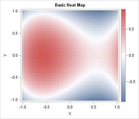
$f(x,y) = x^3 - y^2 - x + 0.5$
A heat map of the function is shown to the right. The function has two critical points at which the gradient is the zero vector: a local maximum at (-1/sqrt(3), 0) and a saddle point at (+1/sqrt(3), 0). The formula for the gradient is grad(f) = [ $3 x^2 - 1$, $-2 y$] and the elements of the Hessian matrix are H[1,1] = 6 x, H[1,2] = H[2,1] = 0, and H[2,2] = -2. You can evaluate these formulas at a specified point to obtain the analytical derivatives at that point.

Finite-difference derivatives in SAS

In SAS, you can use the NLPFDD subroutine in PROC IML to compute finite difference derivatives. (In SAS Viya, you can use the FDDSOLVE subroutine, which is a newer implementation.) By default, the NLPFDD subroutine uses forward-difference formulas to approximate the derivatives. The subroutine returns three output arguments: the value of the function, gradient, and Hessian, respectively, evaluated at a specified point. The following SAS/IML program defines the cubic function and calls the NLPFDD subroutine to approximate the derivatives:

proc iml;
start Func(xy);
   x = xy[,1]; y = xy[,2];
   z = x##3 - y##2 - x + 0.5;
   return( z );
finish;
 
/* Function has local max at (x_max, 0) where x_max = -1/sqrt(3) = -0.57735 */
x_max =  -1/sqrt(3) || 0;
call nlpfdd(f_max, grad_max, Hes_max, "Func", x_max);
 
reset fuzz=2e-6;       /* print 0 for any number less than FUZZ */
print f_max, grad_max, Hes_max;

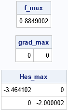
The output shows the value of the function and its derivatives at x₀ = (-1/sqrt(3), 0), which is a local maximum. The value of the function is 0.88. The gradient at the local maximum is the zero vector. The Hessian is a diagonal matrix. The forward-difference derivatives differ from the corresponding analytical values by 2E-6 or less.

Use finite-difference derivatives to classify extrema

One use of the derivatives is to determine whether a point is an extreme value. Points where the gradient of the function vanishes are called critical points. A critical point can be a local extremum or a saddle point. The eigenvalues of the Hessian matrix determine whether a critical point is a local extremum. The eigenvalues are used in the second-derivative test:

1. If the eigenvalues are all positive, the critical point is a local minimum.
2. If the eigenvalues are all negative, the critical point is a local maximum.
3. If some eigenvalues are positive and others are negative, the critical point is a saddle point.
4. If any eigenvalue is zero, the test is inconclusive.

For the current example, the Hessian is a diagonal matrix. By inspection, the eigenvalues are all negative, which proves that the point x₀ = (-1/sqrt(3), 0) is a local maximum. You can repeat the computations for x_s = 1/sqrt(3) || 0, which is a saddle point.

Forward- versus central-difference derivatives

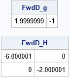
You can evaluate the derivatives at any point, not merely at the critical points. For example, you can evaluate the derivatives of the function at x₁ = (-1, 0.5), which is not an extremum:

x1 = {-1 0.5};
call nlpfdd(FwdD_f, FwdD_g, FwdD_H, "Func", x1);
print FwdD_g, FwdD_H;

By default, the NLPFDD subroutine uses a forward-difference method to approximate the derivatives. You can also use a central difference scheme. The documentation describes six different ways to approximate derivatives, but the most common way is to use the objective function to choose a step size and to use either a forward or central difference. You can use the PAR= keyword to specify the method: PAR[2] = 0 specifies forward difference and PAR[2]=1 specifies central difference:

parm = {.,  00, .};                /* forward diff based on objective function (default) */
call nlpfdd(FwdD_f, FwdD_g, FwdD_H, "Func", x1) par=parm;
parm = {.,  01, .};                /* central diff based on objective function */
call nlpfdd(CenD_f, CenD_g, CenD_H, "Func", x1) par=parm;
 
grad_results = (FwdD_g // CenD_g);
print grad_results[r={"Fwd FD" "Cen FD"} c={"df/dx" "df/dy"}];
HesDiff = FwdD_H - CenD_H;
reset fuzz=2e-16;       /* print small numbers */
print HesDiff;

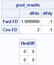
The first table shows the results for the forward-difference method (first row) and the central-difference method (second row). The Hessian matrices are very similar. The output shows that the maximum difference between the Hessians is about 4.5E-7. In general, the forward-difference method is faster but less accurate. The central-difference method is slower but more accurate.

Summary

This article shows how to use the NLPFDD subroutine in SAS/IML to approximate the first-order and second-order partial derivatives of a multivariate function at any point in its domain. The subroutine uses finite-difference methods to approximate the derivatives. You can use a forward-difference method (which is fast but less accurate) or a central-difference method (which is slower but more accurate). The derivatives are useful in many applications, including classifying critical points as minima, maxima, and saddle points.