Isaac Newton had many amazing scientific and mathematical accomplishments. His law of universal gravitation and his creation of calculus are at the top of the list! But in the field of numerical analysis, "Newton's Method" was a groundbreaking advancement for solving for a root of a nonlinear smooth function. The idea of computing derivatives of a function at a point and using them to model the function and predict the location of a root was an ingenious idea. It has been applied to countless applications in the post-Newton era.

As opposed to the Golden Section minimization method, which converges linearly, Newton's method converges quadratically in a neighborhood of a root. This article shows how to program an implementation of Newton's root-finding method in the SAS IML Language. Along the way, we'll mention how to compute numerical derivatives in IML.

Newton's minimization method

Traditionally, Newton's method is a root-finding technique. You are trying to find a point, x_s, such that f(x_s) ≈ 0. In one dimension, you can iterate the sequence x[k+1] = x[k]- f(x)/f'(x), where f' is the first derivative of f, starting from an initial guess.

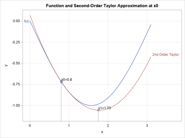
The minimization problem is similar, except now you are searching for a point such that the first derivative vanishes. No problem! Just apply Newton's method to the function f'. Accordingly, you can iterate the sequence x[k+1] = x[k]- f'(x)/f''(x), where f'' is the second derivative of f, starting from an initial guess. This is called Newton's minimization method. Geometrically, the method fits a quadratic function (for example, a parabola) to the graph of the function at the initial guess, as shown in the graph to the right. The next guess is the minimum of that quadratic function.

In practice, professional implementations of Newton's method might take a smaller step, especially when the quantity f'(x)/f''(x) is large relative to x[k]. Often, you will see a step size of α (0 < α ≤ 1), where α is chosen to approximately minimize the objective function in the direction of the step, which becomes α f'(x)/f''(x). This is sometimes called the damped Newton's method.

Newton's minimization method in SAS

You can use the NLPNRA subroutine in SAS IML software to perform nonlinear minimization in any dimension. (Note: NLPNRA is short for "Non-linear Programming: Newton-Raphson".) The NLPNRA subroutine includes step-size control, so it implements a damped Newton's method. To illustrate the technique, let's find the minimum of the function f(x) = -sin(x) on the interval [0,π]. The minimum occurs at π/2 ≈ 1.5707963. The subroutine will compute numerical first and second derivative if you do not specify them explicitly. It is possible to restrict the solution to the interval [0, π], but I will specify an unconstrained problem and hope that my initial guess (x0=0.8) is close enough to the root that Newton's method will converge to π/2. Consequently, the following SAS IML statements approximate the minimum value.

proc iml;
/* 1-D objective function */
start func1D(x);
   return -sin(x);
finish;
 
x0 = 0.8;        /* a starting guess */
call nlpnra(rc, x_min, "func1D", x0) opt={0,4};  /* {0 4} means 'find min' and 'print a lot of output' */
print rc, x_min;

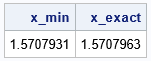
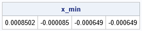
The approximate solution agrees with the exact solution to six digits. In addition to the final solution, you can use ODS output to capture the iteration history of the algorithm. The following output (click to enlarge) summarizes the first four iterations. On the fifth iteration, the algorithm stops and returns the approximate minimum.

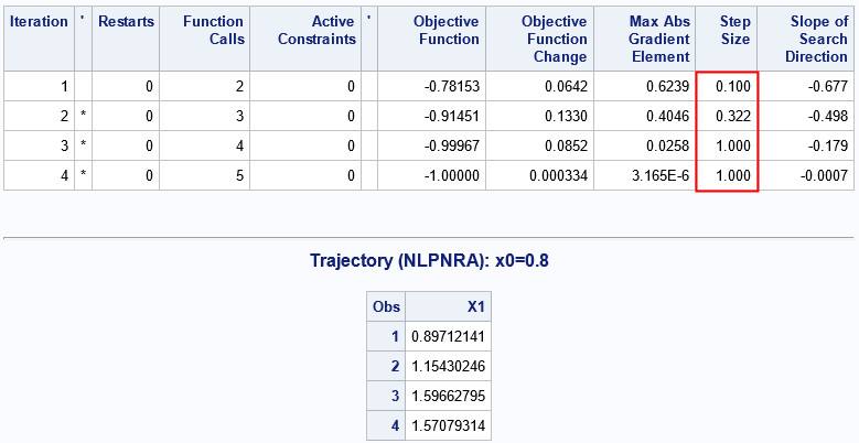
I've highlighted a column of the iteration history table. The column provides the values of α that are used for each step during each iteration in Newton's (damped) minimization method. The second table displays the sequence of approximate solutions, x[1], x[2], x[3], and x[4], which converge to the root at π/2.

Implement Newton's minimization method manually

It is easy to reproduce the iteration history by using the SAS IML language to manually implement Newton's minimization method. You need to evaluate the first and second derivative of the objective function and to specify the step size, α, at each iteration. For simplicity, I'll specify α by copying the values from the iteration history table. The resulting algorithm is simplified version of the computations performed by the NLPNRA subroutine:

start grad(x);
   return -cos(x);
finish;
start hess(x);
   return sin(x);
finish;
 
x0 = 0.8;
alpha = {0.100, 0.322221, 1.000, 1.000};  /* results from line search in NLPNRA */
n_iters = nrow(alpha);
x = j(n_iters+1, 1, .);
x[1] = x0;
/* perform four Newton iterations with the step sizes */
do k = 1 to n_iters;
   H = hess(x[k]);
   G = grad(x[k]);
   x[k+1] = x[k] - alpha[k]* G / H;  /* 1-d solution */
end;
print x[rowname=(0:n_iters)];

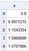
The iterations of this hard-coded 1-D implementation agree with the results of the NLPNRA subroutine for this example. The next section generalizes the implementation to arbitrary dimensions but does not try to use a modified step size.

Generalizing Newton's minimization method

If you are familiar with multivariate calculus, you can generalize the Newton minimization method to work in higher dimensions:

• Instead of finding a point where the first derivative of a 1-D function vanishes, we seek a point such that the gradient vector, G, (the vector of partial derivatives) is the zero vector.
• Instead of using the second derivative of a 1-D function, we use the Hessian matrix, H, (the matrix of second partial derivatives) to estimate the curvature of the function at each iteration.
• In 1-D, the step is based on the ratio δ = f'/f''. Recast that equation to find a value of δ such that f''(x)*δ = f'(x). The generalization to higher dimensions is to find a vector, δ, such that H*δ = G. We then step in the direction of δ to find the next term in the sequence of approximations.

The method of determining an optimal step size, is a little complicated. Therefore, the following implementation of Newton's method always takes a full step. That is, it is not the damped method. Because of this, the output of this function will not always match the output of the NLPNRA subroutine. However, this function implements the main ideas behind Newton's method in higher dimensions. Because it is tedious to write modules that evaluate the gradient and Hessian of the objective function, this implementation uses the NLPFDD function in SAS IML to obtain finite-difference derivatives.

/* This user-defined function is similar to the built-in NLPNRA subroutine,
   but this version always takes a full step size, which might lead to instabilities.
   Also, NLPNRA considers other stopping criteria, such as whether |f(x[k+i])-f(x[k])| is small. */
start NewtonMinMethod(funcName, x0, tolerance=1e-5, maxIters=100);
   x  = x0;   /* x[k+1] */
   xk = .;    /* x[k]   */
   do i = 1 to maxIters until( norm(x-xk) < tolerance );
      xk = x;
      call nlpfdd(f, G, H, funcName, xk);
      delta = solve(H, -G`);
      x = xk + delta`; /* take full step; to match NLPNRA, use alpha*delta where alpha <=1 */
   end;
   return x;
finish;
 
x0 = 0.8;
x_min = NewtonMinMethod("FUNC1D", x0);  /* pass the name of the objective function as a string */
x_exact = constant('pi')/2;
print x_min x_exact;

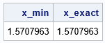
The example shows that although the NewtonMinMethod function is written to solve minimizations in any dimension, it still works for 1-D functions. The following example shows that the same function also works for a function of four variables:

/* define the Powell function in 4-D */
start func4D(x);
   return (x[1]+10*x[2])##2 + 5*(x[3]-x[4])##2 + (x[2]-2*x[3])##4 + 10*(x[1]-x[4])##4;
finish;
 
/* the same code works in higher dimensions */
x0 = {3 -1 0 1};           /* initial guess */
x_min = NewtonMinMethod("FUNC4D", x0);
print x_min;

A comment on step sizes

Newton's minimization method works well when the function near the minimum looks somewhat like a quadratic function. As is evident from the mathematical expression for the Newton iteration, this method in 1-D cannot proceed when the second derivative evaluates to zero. For example, if the iteration lands on an inflection point, the second derivative there vanishes. In higher dimensions, it cannot proceed when the Hessian matrix is singular at a point. Geometrically, the curvature of the function is zero along some direction.

Even if the algorithm does not exactly encounter an inflection point, nearby points can also cause problems. If the curvature is relatively small and the gradient is not zero, then the 1-D step f'(x)/f''(x) can be arbitrarily large. That means that the next candidate for the minimum will be far away from the previous candidate.

In the simple 1-D example f(x) = -sin(x), the function has an inflection point at x=0. Consequently, if you start near x=0, the next iteration could be far away. For example, let's take one step starting from the point x0=0.1:

/* If you guess x0 where the curvature is small, Newton's method (without step-size control) can step far away. */
x0 = 0.1;
x1 = NewtonMinMethod("FUNC1D", x0, 1e-5, 1); /* 1 iteration */
print x1;

The second iterate is 10 units away from the initial guess. Because the sine function is periodic, Newton's method in this case will find the minimum at x=7π/2 ≈ 11. However, in general, large steps will result in a new iterate that is far away from the previous one, which violates the concept of searching "near" a certain guess. Some implementations of Newton's method might have step-size controls to prevent this behavior.

Summary

This article explains Newton's method for finding the minimum of a function. The method iteratively refines a guess by using first and second derivatives (or the gradients and Hessians in higher dimensions). In SAS, you can use the built-in NLPNRA subroutine in SAS IML to perform Newton's minimization in any dimension. The article shows how to implement a simple version of Newton's method in PROC IML so that you can see the main ideas. The simple implementation lacks step-size control, which can avoid instabilities in the minimization.