Newton's method was in the news this week. Not the well-known linear method for finding roots, but a more complicated method for finding minima, sometimes called the method of successive parabolic approximations. Newton's parabolic method was recently improved by modern researchers who extended the method to use higher-dimensional polynomials.

The news caused me to think about one-dimensional minimization. In SAS, you can select from many algorithms that enable you to find a minima for a function. These algorithms work in 1-D, 2-D, and higher dimensions. They are often used in conjunction with maximum likelihood estimation to fit models to data. Many of these algorithms (for example, the Newton-Raphson algorithm) converge super-linearly.

One method that is not included in the SAS library is the Golden Section search algorithm. This method is limited to finding a minimum of a 1-D function on a closed interval. The name "Golden Section" is used because at each iteration the width of the interval that bounds the minimum decreases by a factor of 1/φ at each step, where φ = (1 + sqrt(5))/ 2 is the golden ratio. (Note: 1/φ ≈ 0.618.) The Golden Section search is sometimes used as part of other iterative methods when you need to step in a certain direction in parameter space (think, gradient descent), so it is useful to know about. It is guaranteed to find an approximate minima for a unimodal function on an interval.

This article uses SAS/IML to create a function that performs the Golden Section search to find the minimum of a 1-D function on a closed interval. Along the way, I'll make a few comparisons about the syntax of Python and also about linear versus super-linear convergence.

Converting Python to IML syntax

It is often said that if you know how to program in one language, it is relatively easy to learn additional languages. That is because the main programming constructs are common to all languages; only the syntax differs. If you know how to use loops, function, if/then statements, and so forth, you can start to program in any language by learning to write those building blocks.

When I decided to write about this topic, I went to the Wikipedia entry for the Golden Section search. The entry includes a Python program that implements a simple version of the Golden Section search. Here is the Python program, with block comments removed:

import math
 
invphi = (math.sqrt(5) - 1) / 2  # 1 / phi
 
def gss(f, a, b, tolerance=1e-5):
    while b - a > tolerance:
        c = b - (b - a) * invphi
        d = a + (b - a) * invphi
        if f(c) < f(d):
            b = d
        else:  
            a = c
 
    return (b + a) / 2       # x that minimizes f on the original [a,b] interval

Programmers in SAS, SAS/IML, C/C++ and other languages will easily be able to read this program. The gss() function (gss = golden section search) takes three required parameters and one optional parameter. The required parameters are an objective function (f), and the endpoints of a 1-D interval [a,b]. The optional parameter is a tolerance, which you can use to specify how closely you want to approximate the solution. Assuming that f is unimodal on [a,b], the function returns an approximation for the value of x that minimizes f on the interval. It does this by "testing" the program at new points (c and d) in the interval and decreasing the width of the interval at each step, making sure at each step that the minimum remains inside the interval.

Although I could have reused the Golden Section search function on pp. 85-86 of Wicklin (2010, Statistical Programming with SAS/IML Software), I thought it might be instructive to convert the Python program to a equivalent SAS program in PROC IML. Because I program in both languages, I could quickly translate the program from Python to IML. Here is my conversion:

proc iml;
 
start gss(ab, tolerance=1e-5);
    invphi = (sqrt(5) - 1) / 2;  /* 1 / phi */
    a = ab[1]; b = ab[2];
    do while (b - a > tolerance);
        c = b - (b - a) * invphi;
        d = a + (b - a) * invphi;
        if func(c) < func(d) then
            b = d;
        else   /* f(c) > f(d) to find the maximum */
            a = c;
    end;
    return (b + a) / 2;
finish;

The main changes are:

• SAS statements must end with a semi-colon.
• SAS does not require that you import a math library. I changed function calls such as math.sqrt() to the SAS equivalent, such as SQRT.
• The example defines a global variable (invphi) that is accessed from inside the gss() function. I defined a local variable inside the function.
• Python functions are defined by using the def keyword. A colon indicates the end of the signature. Indenting determines the end of the function definition. In contrast, SAS/IML functions are defined by using a START/FINISH pair of keywords.
• I decided to pass in an interval (a 1x2 row vector, ab) instead of two endpoints (a and b). Not only does this match the syntax for other functions in IML (for example, QUAD and FROOT) that use intervals, but also IML passes parameters by reference, not by value. The function updates the value of the a and b parameters. If I pass in a and b, those values will change in the main scope, which might be an undesirable side effect of calling the function.
• Python uses triple quotes for block comments and the '#' character for in-line comments. I changed all comments to the SAS block comment: /* comment */.
• I changed Python's while loop to a DO WHILE loop. Whereas Python uses indenting to show the end of the loop, in SAS you need to use a DO/END block.
• I replaced the Python if/else statement with the IF-THEN syntax in SAS. If necessary, I would use a DO/END block to execute multiple statements.
• I hard-coded the name of the objective function as FUNC. The Python program passed the function name as a parameter to the function. I really like the fact that in Python everything is an object, and you can pass any object to functions.

To show that the function works, the following statements define the FUNC function as f(x) = -sin(x), which has a minimum value at π / 2 on the interval [0,3]. By default, the x value that achieves the minimum is found to within 1E-5.

start func(x);
    return -sin(x);
finish;
 
x_min = gss( {0 3} );
true_min = constant('pi')/2;
print x_min true_min;

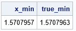
As promised, the IML routine finds the minimum to an accuracy within 1E-5 of the true value.

Rate of convergence

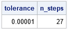
The Golden Section search finds the root to within a tolerance of δ It isn't hard to compute how many iterations are required to achieve the tolerance. Let r = 1/φ be the inverse of the Golden Ratio. If h is the width of the initial search interval, the width of the next interval is h*r = 0.618*h. Thus, the width of the interval after n steps is h*rⁿ. We want to find the value of n for which h*rⁿ < δ. Taking logs, this occurs when n*log(r) < log(δ/h). Because r <1, log(r) is negative. Therefore, the interval will be smaller than δ when n ≥ log(δ/h) / log(r). For our example, the initial interval had a width of h=3. The following calculation shows that the iteration requires 27 iterations:

/* number of steps to find min to precision 'tolerance' if initial interval has width h */
h = 3;                            /* width of [0,3] interval */
tolerance = 1e-5;
r = (sqrt(5) - 1) / 2;            /* 1 / phi */
n_steps = ceil( log10(tolerance/h) / log10(r) );
print tolerance n_steps;

From the formula, you can see that the number of steps required by the Golden Section search is proportional to the logarithm (for any base) of the tolerance. You can graph the number of steps versus the log of the tolerance to visualize how this algorithm behaves as you tighten the tolerance.

/* plot number of steps versus size of tolerance */
pow = do(-9, -4, 0.01);
tol =  10##pow;
h = 1;
n_steps = ceil( log10(tol/h) / log10(invphi) );
 
title "Number of steps to convergence within a desired tolerance";
title2 "Assume initial interval has unit length";
call series(pow, n_steps) grid={x y} label={'log10(Tolerance)' 'Number of Iterations'};

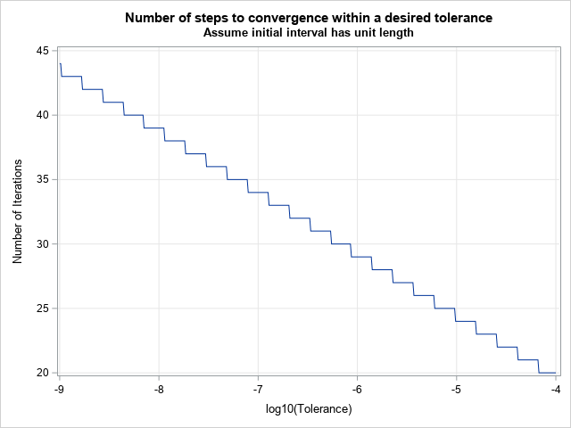
For an initial interval that has unit width, it takes 20 steps to converge to 4 decimal places and twice as many (40) to converge to 8 decimal digits. The graph shows that the Golden Section search exhibits a linear rate of convergence, which is not very fast when compared to other minimization methods that converge super-linearly. However, the Golden Section search has an important advantage: it never fails to find the minimum of a unimodal function on a closed interval. That is because the minimum is bracketed at each step.

Summary

An important 1-D minimization method that is often taught in school is the Golden Section search. This method will find the minimum of a unimodal 1-D function on a closed interval. For this example, it was straightforward to convert a Python implementation to a SAS/IML program. I called the function on an example and demonstrated that the number of iterations is a linear function of the precision of the computation. By the way, if you want to fid a maximum of a unimodal function, g(x), just find the minimum of -g(x).