A recent article about how to estimate a two-dimensional distribution function in SAS inspired me to think about a related computation: a 2-D cumulative sum. Suppose you have numbers in a matrix, X. A 2-D cumulative sum is a second matrix, C, such that the C[p,q] gives the sum of the cells of X for rows less than p and columns less than q. In symbols, C[p,q] = sum( X[i,j], i ≤ p, j ≤ q ).

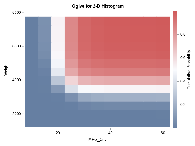
This article shows a clever way to compute a 2-D cumulative sum and shows how to use this computation to compute a 2-D ogive, which is a histogram-based estimate of a 2-D cumulative distribution (CDF). An example of a 2-D ogive is shown to the right. You can compare the ogive to the 2-D CDF estimate from the previous article.

2-D cumulative sums

A naive computation of the 2-D cumulative sums would use nested loops to sum submatrices of X. If X is an N x M matrix, you might think that the cumulative sum requires computing N*M calls to the SUM function. However, there is a simpler computation that requires only N+M calls to the CUSUM function. You can prove by induction that the following algorithm gives the cumulative sums:

1. Compute the cumulative sums for each row. In a matrix language such as SAS/IML, this requires N calls to the CUSUM function.
2. Use the results of the first step and compute the "cumulative sums of the cumulative sums" down the columns. This requires M calls to the CUSUM function.

Thus, in the SAS/IML language, a 2-D cumulative sum algorithm looks like this:

proc iml;
/* compute the 2-D CUSUM */
start Cusum2D(X);
   C = j(nrow(X), ncol(X), .);  /* allocate result matrix */
   do i = 1 to nrow(X);
      C[i,] = cusum( X[i,] );   /* cusum across each row */
   end;
   do j = 1 to ncol(X);
      C[,j] = cusum( C[,j] );   /* cusum down columns */
   end;
   return C;
finish;
store module=(Cusum2D);
 
Count = { 7  6 1 3,
          6  3 5 2,
          1  2 4 1};
Cu = Cusum2D(Count);
print Count, Cu;

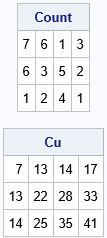
The output shows the original matrix and the 2-D cumulative sums. For example, in the CU matrix, the (2,3) cell contains the sum of the submatrix Count[1:2, 1:3]. That is, the value 28 in the CU matrix is the sum (7+6+1+6+3+5) of values in the Count matrix.

From cumulative sums to ogives

Recall that an ogive is a cumulative histogram. If you start with a histogram that shows the number of observations (counts) in each bin, then an ogive displays the cumulative counts. If you scale the histogram so that it estimates the probability density, then the ogive estimates the univariate CDF.

A previous article showed how to construct an ogive in one dimension from the histogram. To construct a two-dimensional ogive, do the following:

• You start with a 2-D histogram. For definiteness, let's assume that the histogram displays the counts in each two-dimensional bin.
• You compute the 2-D cumulative sums, as shown in the previous section. If you divide the cumulative sums by the total number of observations, you obtain the cumulative proportions.
• The matrix of cumulative proportions is the 2-D ogive. However, by convention, an ogive starts at 0. Consequently, you should append a row and column of zeros to the left and top of the matrix of bin counts.

You can download the complete SAS/IML program that computes the ogive. The program defines two SAS/IML functions. The Hist2D function creates a matrix of counts for bivariate data. The Ogive2D function takes the matrix of counts and converts it to a matrix of cumulative proportions by calling the Cusum2D function in the previous section. It also pads the cumulative proportions with a row and a column of zeros. The function returns a SAS/IML list that contains the ogive and the vectors of endpoints for the ogive. The following statements construct an ogive from the bivariate data for the MPG_City and Weight variables in the Sashelp.Cars data set:

proc iml;
/* load computational modules */
load module=(Hist2D Cusum2D Ogive2D);
 
/* read bivariate data */
use Sashelp.Cars;
   read all var {MPG_City Weight} into Z;
close;
 
* define cut points in X direction (or use the GSCALE function);
cutX = do(10, 60, 5);        
cutY = do(1500, 7500, 500);
Count = Hist2D(Z, cutX, cutY);   /* matrix of counts in each 2-D bin */
L = Ogive2D(Count, cutX, cutY);  /* return value is a list */
ogive = L$'Ogive';               /* matrix of cumulative proportions */
print ogive[F=Best5. r=(L$'YPts') c=(L$'XPts')];

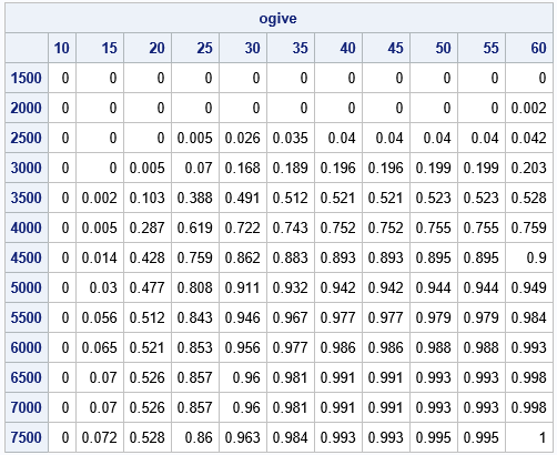
The table shows the values of the ogive. You could use bilinear interpolation if you want to estimate the curve that corresponds to a specific probability, such as 0.5. You can also visualize the ogive by using a heat map, as shown at the top of this article. Notice the difference between the tabular and graphical views: rows increase DOWN in a matrix, but the Y-axis points UP in a graph. To compare the table and graph, you can reverse the rows of the table.

Summary

This article shows how to compute a 2-D cumulative sum. You can use the 2-D cumulative sum to create a 2-D ogive from the counts of a 2-D histogram. The ogive is a histogram-based estimate of the 2-D CDF. You can download the complete SAS program that computes 2-D cumulative sums, histograms, and ogives.