Last Monday I discussed how to choose the bin width and location for a histogram in SAS. The height of each histogram bar shows the number of observations in each bin. Although my recent article didn't mention it, you can also use the IML procedure to count the number of observations in each bin. The BIN function associates a bin to each observation, and the TABULATE subroutine computes the count for each bin. I have previously blogged about how to use this technique to count the observations in bins of equal or unequal width.
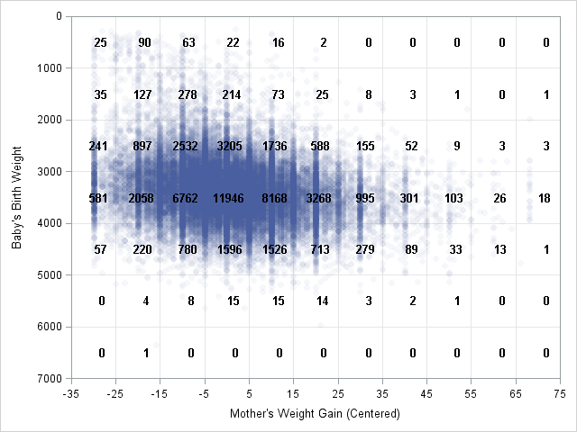
You can also count the number of observations in two-dimensional bins. Specifically, you can divide the X direction into kx bins, divide the Y direction into ky bins, and count the number of observations in each of the kx x ky rectangles. In a previous article, I described how to bin 2-D data by using the SAS/IML language and produced the scatter plot at the left. The graph displays the birth weight of 50,000 babies versus the relative weight gain of their mothers for data in the Sashelp.bweight data set.
I recently remembered that you can also count observations in 2-D bins by using the KDE procedure. The BIVAR statement in the KDE procedure supports an OUT= option, which writes a SAS data set that contains the counts in each bin. You can specify the number of bins in each direction by using the NGRID= option on the BIVAR statement, as shown by the following statements:
ods select none; proc kde data=sashelp.bweight; bivar MomWtGain(ngrid=11) Weight(ngrid=7) / out=KDEOut; run; ods select all; proc print data=KDEOut(obs=10 drop=density); run; |
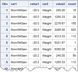
As shown in the output, the the VALUE1 and VALUE2 variables contain the coordinates of the center of each bin. The COUNT variable contains the bin count. You can read the counts into SAS/IML and print it out as a matrix. In the data set, the Y variable changes the fastest as you go down the rows. Consequently, you need to use the SHAPECOL function rather than the SHAPE function to form the 7 x 11 matrix of counts:
proc iml; kX = 11; kY = 7; use KDEOut; read all var {Value1 Value2 Count}; close; M = shapecol(Count, kY, kX); /* reshape into kY x kX matrix */ /* create labels for cells in X and Y directions */ idx = do(1,nrow(Value1),kY); /* location of X labels */ labelX = putn(Value1[idx], "5.1"); labelY = putn(Value2[1:kY], "5.0"); print M[c=labelX r=labelY]; |
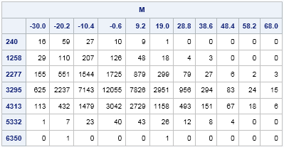
As I explained in Monday's blog post, there are two standard ways to choose bins for a histogram: the "midpoints" method and the "endpoints" method. If you compare the bin counts from PROC KDE to the bin counts from my SAS/IML program, you will see small differences. That is because the KDE procedure uses the "midpoints" algorithm for subdividing the data range, whereas I used the "endpoints" algorithm for my SAS/IML program.
Last week I showed how to use heat maps to visualize matrices in SAS/IML. This matrix of counts is begging to be visualized with a heat map. Because the counts vary across several orders of magnitude (from 100 to more than 104), a linear color ramp will not be an effective way to visualize the raw counts. Instead, transform the counts to a log scale and create a heat map of the log-counts:
call HeatmapCont(log10(1+M)) xvalues=labelX yvalues=labelY colorramp="ThreeColor" legendtitle="Log(Count)" title="Counts in Each Bin"; |
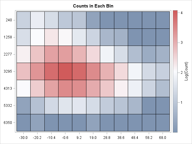
The heat map shows the log-count of each bin. If you prefer a light-to-dark heatmap for the density, use the "TwoColor" value for the COLORRAMP= option. The heat map is a great way to see the distribution of counts at a glance. It enables you to see the approximate values of most cells, and you can easily determine cells where there are many or few observations. Of course, if you want to know the exact value of the count in each rectangular cell, look at the tabular output.

4 Comments
Pingback: How to create a hexagonal bin plot in SAS - The DO Loop
Pingback: Designing a quantile bin plot - The DO Loop
Hi
Part of my research is to create a code that compute the kernel density estimation. I managed to creat my code but when I tried to extend it I couldn't.
HOW can I repeat this process as many as 1000 times and save the results in a matrix that is 100 X 1000???? what i mean is that I need 100 grids for every simulation
Below is my code:
proc iml;
...
Thanks
Majdi
You can ask questions like this at the
SAS/IML Support Community. You can search my blog for similar simulations in SAS/IML.