This article shows how to perform two-dimensional bilinear interpolation in SAS by using a SAS/IML function. It is assumed that you have observed the values of a response variable on a regular grid of locations.

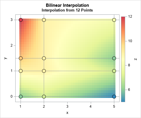
A previous article showed how to interpolate inside one rectangular cell. When you have a grid of cells and a point (x, y) at which to interpolate, the first step is to efficiently locate which cell contains (x, y). You can then use the values at the corners of the cell to interpolate at (x, y), as shown in the previous article. For example, the adjacent graph shows the bilinear interpolation function that is defined by 12 points on a 4 x 3 grid.

You can download the SAS program that creates the analyses and graphs in this article.

Bilinear interpolation assumptions

For two-dimensional linear interpolation of points, the following sets of numbers are the inputs for bilinear interpolation:

1. Grid locations: Let x1 < x2 < ... < xp be the horizontal coordinates of a regular grid. Let y1 < y2 < ... < yn be the vertical coordinates.
2. Response Values: Let Z be an n x p matrix of response values on the grid. The (j, i)th value of Z is the response value at the location (xi, yj). Notice that the columns of Z correspond to the horizontal positions for the X values and the rows of Z correspond to the vertical positions for the Y values. (This might seem "backwards" to you.) The response values data should not contain any missing values. The X, Y, and Z values (called the "fitting data") define the bilinear interpolation function on the rectangle [x1, xp] x [y1, yn].
3. Values to score: Let (s1, t1), (s2, t2), ..., (sk, tk) be a set of k new (x, y) values at which you want to interpolate. All values must be within the range of the data: x1 ≤ s_i ≤ xp and y1 ≤ s_i ≤ yn for all (i,j) pairs. These values are called the "scoring data" or the "query data."

The goal of interpolation is to estimate the response at each location (s_i, t_j) based on the values at the corner of the cell that contains the location. I have written a SAS/IML function called BilinearInterp, which you can freely download and use. The following statements indicate how to define and store the bilinearInterp function:

proc iml;
/* xGrd : vector of Nx points along x axis
   yGrd : vector of Ny points along y axis
   z    : Ny x Nx matrix. The value Z[i,j] is the value at xGrd[j] and yGrd[i]
   t    : k x 2 matrix of points at which to interpolate
   The function returns a k x 1 vector, which is the bilinear interpolation at each row of t. 
*/
start bilinearInterp(xgrd, ygrd, z, t);
   /* download function from 
      https://github.com/sascommunities/the-do-loop-blog/blob/master/interpolation/bilinearInterp.sas 
   */
finish;
store module=bilinearInterp;       /* store the module so it can be loaded later */
QUIT;

You only need to store the module one time. You then load the module in any SAS/IML program that needs to use it. You can learn more about storing and loading SAS/IML modules.

The structure of the fitting data

The fitting data for bilinear interpolation consists of the grid of points (Z) and the X and Y locations of each grid point. The X and Y values do not need to be evenly spaced, but they can be.

Often the fitting data are stored in "long form" as triplets of (X, Y, Z) values. If so, the first step is to read the triplets and convert them into a matrix of Z values where the columns are associated with the X values and the rows are associated with the Y values. For example, the following example data set specifies a response variable (Z) on a 4 x 3 grid. The values of the grid in the Y direction are {0, 1, 1.5, 3} and the values in the X direction are {1, 2, 5}.

As explained in the previous article, the data must be sorted by Y and then by X. The following statements read the data into a SAS/IML matrix and extract the grid points in the X and Y direction:

data Have;
input x y z;
datalines;
1 0   6 
2 0   7 
5 0   5 
1 1   9 
2 1   9 
5 1   7 
1 1.5 10 
2 1.5 9 
5 1.5 6 
1 3   12 
2 3   9 
5 3   8 
;
 
/* If the data are not already sorted, sort by Y and X */
proc sort data=Have; by Y X; run; 
 
proc iml;
use Have; read all var {x y z}; close;
xGrd = unique(x);                      /* find grid points */                     
yGrd = unique(y);
z = shape(z, ncol(yGrd), ncol(xGrd)); /* data must be sorted by y, then x */
print z[r=(char(yGrd)) c=(char(xGrd))];

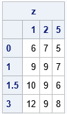
Again, note that the columns of Z represent the X values and the rows represent the Y values. The xGrd and yGrd vectors contain the grid points along the horizontal and vertical dimensions of the grid, respectively.

The structure of the scoring data

The bilinearInterp function assumes that the points at which to interpolate are stored in a k x 2 matrix. Each row is an (x,y) location at which to interpolate from the fitting data. If an (x,y) location is outside of the fitting data, then the bilinearInterp function returns a missing value. The scoring locations do not need to be sorted.

The following example specifies six valid points and two invalid interpolation points:

t = {0   0,     /* not in data range */
     1   1,
     1   2,
     2.5 2,
     4   0.5,
     4   2,
     5   3,
     6   3};    /* not in data range */
 
/* LOAD the previously stored function */
load module=bilinearInterp;  
F = bilinearInterp(xGrd, yGrd, z, t);
print t[c={'x' 'y'}] F[format=Best4.];

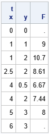
The grid is defined on the rectangle [1,5] x [0,3]. The first and last rows of t are outside of the rectangle, so the interpolation returns missing values at those locations. The locations (1,1) and (5,3) are grid locations (corners of a cell), and the interpolation returns the correct response values. The other locations are in one of the grid cells. The interpolation is found by scaling the appropriate rectangle onto the unit square and applying the bilinear interpolation formula, as shown in the previous article.

Visualizing the bilinear interpolation function

You can use the ExpandGrid function to generate a fine grid of locations at which to interpolate. You can visualize the bilinear interpolation function by using a heat map or by using a surface plot.

The heat map visualization is shown at the top of this article. The colors indicate the interpolated values of the response variable. The markers indicate the observed values of the response variable. The reference lines show the grid that is defined by the fitting data.

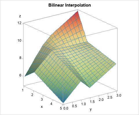
The following graph visualizes the interpolation function by using a surface plot. The function is piecewise quadratic. Within each cell, it is linear on lines of constant X and constant Y. The "ridge lines" on the surface correspond to the locations where two adjacent grid cells meet.

Summary

In summary, you can perform bilinear interpolation in SAS by using a SAS/IML function. The function uses fitting data (X, Y, and Z locations on a grid) to interpolate. Inside each cell, the interpolation is quadratic and is linear on lines of constant X and constant Y. For each location point, the interpolation function first determines what cell the point is in. It then uses the corners of the cell to interpolate at the point. You can download the SAS program that performs bilinear interpolation and generates the tables and graphs in this article.