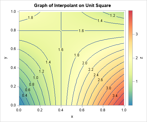
I've previously written about linear interpolation in one dimension. Bilinear interpolation is a method for two-dimensional interpolation on a rectangle. If the value of a function is known at the four corners of a rectangle, an interpolation scheme gives you a way to estimate the function at any point in the rectangle's interior. Bilinear interpolation is a weighted average of the values at the four corners of the rectangle. For an (x,y) position inside the rectangle, the weights are determined by the distance between the point and the corners. Corners that are closer to the point get more weight. The generic result is a saddle-shaped quadratic function, as shown in the contour plot to the right.

The Wikipedia article on bilinear interpolation provides a lot of formulas, but the article is needlessly complicated. The only important formula is how to interpolate on the unit square [0,1] x [0,1]. To interpolate on any other rectangle, simply map your rectangle onto the unit square and do the interpolation there. This trick works for bilinear interpolation because the weighted average depends only on the relative position of a point and the corners of the rectangle. Given a rectangle with lower-left corner (x0, y0) and upper right corner (x1, y1), you can map it into the unit square by using the transformation (x, y) → (u, v) where u = (x-x0)/(x1-x0) and v = (y-y0)/(y1-y0).

Bilinear interpolation on the unit square

Suppose that you want to interpolate on the unit square. Assume you know the values of a continuous function at the corners of the square:

• z00 is the function value at (0,0), the lower left corner
• z10 is the function value at (1,0), the lower right corner
• z01 is the function value at (0,1), the upper left corner
• z11 is the function value at (1,1), the upper right corner

If (x,y) is any point inside the unit square, the interpolation at that point is the following weighted average of the values at the four corners:
F(x,y) = z00*(1-x)*(1-y) + z10*x*(1-y) + z01*(1-x)*y + z11*x*y

Notice that the interpolant is linear with respect to the values of the corners of the square. It is quadratic with respect to the location of the interpolation point. The interpolant is linear along every horizontal line (lines of constant y) and along every vertical line (lines of constant x).

Implement bilinear interpolation on the unit square in SAS

Suppose that the function values at the corners of a unit square are z00 = 0, z10 = 4, z01 = 2, and z11 = 1. For these values, the bilinear interpolant on the unit square is shown at the top of this article. Notice that the value of the interpolant at the corners agrees with the data values. Notice also that the interpolant is linear along each edge of the square. It is not easy to see that the interpolant is linear along each horizontal and vertical line, but that is true.

In SAS, you can use the SAS/IML matrix language to define a function that performs bilinear interpolation on the unit square. The function takes two arguments:

• z is a four-element that specifies the values of the data at the corners of the square. The values are specified in the following order: lower left, lower right, upper left, and upper right. This is the "fitting data."
• t is a k x 2 matrix, where each row specifies a point at which to interpolate. This is the "scoring data."

In a matrix language such as SAS/IML, the function can be written in vectorized form without using any loops:

proc iml;
start bilinearInterpSquare(z, t);
   z00 = z[1]; z10 = z[2]; z01 = z[3]; z11 = z[4]; 
   x = t[,1];  y = t[,2];
   cx = 1-x;                    /* cx = complement of x */
   return( (z00*cx + z10*x)#(1-y) + 
           (z01*cx + z11*x)#y );
finish;
 
/* specify the fitting data */
z = {0 4,                       /* bottom: values at (0,0) and (1,0) */
     2 1};                      /* top: values at (0,1) and (1,1) */
print z[c={'x=0' 'x=1'} r={'y=0' 'y=1'}];
 
t = {0.5 0,                     /* specify the scoring data */
     0    0.25,
     1    0.66666666,
     0.5  0.75,
     0.75 0.5     };
F = bilinearInterpSquare(z, t); /* test the bilinear interpolation function */
print t[c={'x' 'y'} format=FRACT.] F;

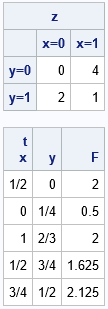
For points on the edge of the square, you can check a few values in your head:

• The point (1/2, 0) is halfway between the corners with values 0 and 4. Therefore the interpolation gives 2.
• The point (0, 1/4) is a quarter of the way between the corners with values 0 and 2. Therefore the interpolation gives 0.5.
• The point (1, 2/3) is two thirds of the way between the corners with values 4 and 1. Therefore the interpolation gives 2.

The other points are in the interior of the square. The interpolant at those points is a weighted average of the corner values.

Visualize the interpolant function

Let's use the bilinearInterpSquare function to evaluate a grid of points. You can use the ExpandGrid function in SAS/IML to generate a grid of points. When we look at the values of the interpolant on a grid or in a heat map, we want the X values to change for each column and the Y values to change for each row. This means that you should reverse the usual order of the arguments to the ExpandGrid function:

/* for visualization, reverse the arguments to ExpandGrid and then swap 1st and 2nd columns of t */
xGrd = do(0, 1, 0.2);
yGrd = do(0, 1, 0.2);
t = ExpandGrid(yGrd, xGrd);  /* want X changing fastest; put in 2nd col */
t = t[ ,{2 1}];              /* reverse the columns from (y,x) to (x,y) */
F = bilinearInterpSquare(z, t);
Q = shape(F, ncol(yGrd), ncol(xGrd));
print Q[r=(char(YGrd,3)) c=(char(xGrd,3)) label="Bilinear Interpolant"];

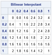
The table shows the interpolant evaluated at the coordinates of a regular 6 x 6 grid. The column headers give the coordinate of the X variable and the row headers give the coordinates of the Y variable. You can see that each column and each row is an arithmetic sequence, which shows that the interpolant is linear on vertical and horizontal lines.

You can use a finer grid and a heat map to visualize the interpolant as a surface. Notice that in the previous table, the Y values increase as you go down the rows. If you want the Y axis to point up instead of down, you can reverse the rows of the grid (and the labels) before you create a heat map:

/* increase the grid resolution and visualize by using a heat map */
xGrd = do(0, 1, 0.1);
yGrd = do(0, 1, 0.1);
t = ExpandGrid(yGrd, xGrd);  /* want X changing fastest; put in 2nd col */
t = t[ ,{2 1}];              /* reverse the columns from (y,x) to (x,y) */
F = bilinearInterpSquare(z, t);
Q = shape(F, ncol(yGrd), ncol(xGrd));
 
/* currently, the Y axis is pointing down. Flip it and the labels. */
H = Q[ nrow(Q):1, ];
reverseY = yGrd[ ,ncol(yGrd):1];
call heatmapcont(H) range={0 4} displayoutlines=0
     xValues=xGrd yValues=reverseY
     colorramp=palette("Spectral", 7)[,7:1]
     title="Interpolation at Multiple Points in the Unit Square";

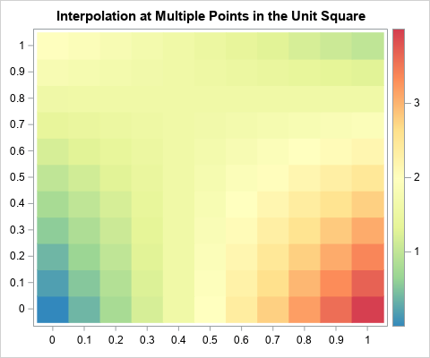
The heat map agrees with the contour plot at the top of this article. The heat map also makes it easier to see that the bilinear interpolant is linear on each row and column.

In summary, you can create a short SAS/IML function that performs bilinear interpolation on the unit square. (You can download the SAS program that generates the tables and graphs in this article.) The interpolant is a quadratic saddle-shaped function inside the square. You can use the ideas in this article to create a function that performs bilinear interpolation on an arbitrary grid of fitting data. The next article shows a general function for bilinear interpolation in SAS.