Linear interpolation in SAS

SAS programmers sometimes ask about ways to perform one-dimensional linear interpolation in SAS. This article shows three ways to perform linear interpolation in SAS: PROC IML (in SAS/IML software), PROC EXPAND (in SAS/ETS software), and PROC TRANSREG (in SAS/STAT software). Of these, PROC IML Is the simplest to use and has the most flexibility. This article shows how to implement an efficient 1-D linear interpolation algorithm in SAS. You can download the SAS program that creates the analyses and graphs in this article.

Linear interpolation assumptions

For one-dimensional linear interpolation of points in the plane, you need two sets of numbers:

Data: Let (x1, y1), (x2, y2), ..., (xn, yn) be a set of n data points. The data should not contain any missing values. The data must be ordered so that x1 < x2 < ... < xn. These values uniquely define the linear interpolation function on [x1, xn]. I call this the "sample data" or "fitting data" because it is used to create the linear interpolation model.
Values to score: Let {t1, t2, ..., tk} be a set of k new values for the X variable. For interpolation, all values must be within the range of the data: x1 ≤ t_i ≤ xn for all i. The goal of interpolation is to produce a new Y value for each value of t_i. The scoring data is also called the "query data."

Interpolation requires a model. For linear interpolation, the model is the unique piecewise linear function that passes through each sample point and is linear on each interval [x_i, x_i+1]. The model is usually undefined outside of the range of the data, although there are various (nonunique) ways to extrapolate the model beyond the range of the data. You fit the model by using the data. You then score the model on the set of new values.

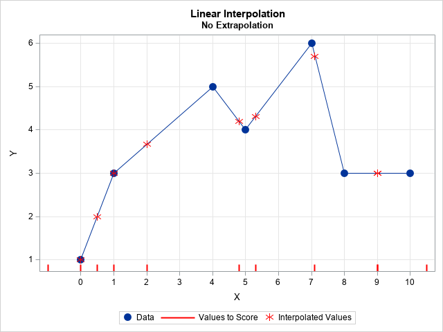
The following SAS data sets define example data for linear interpolation. The POINTS data set contains fitting data that define the linear model. The SCORE data set contains the new query points at which we want to interpolate. The linear interpolation is shown to the right. The sample data are shown as blue markers. The model is shown as blue lines. The query values to score are shown as a fringe plot along the X axis. The interpolated values are shown as red markers.

The data used for this example are:

/* Example data for 1-D interpolation */
data Points;  /* these points define the model */
input x y;
datalines;
0  1
1  3
4  5
5  4
7  6
8  3
10 3
;
 
data Score; /* these points are to be interpolated */
input t @@;
datalines;
2 -1 4.8 0 0.5 1 9 5.3 7.1 10.5 9
;

For convenience, the fitting data are already sorted by the X variable, which is in the range [0, 10]. The scoring data set does not need to be sorted.

The scoring data for this example contains five special values:

Two scoring values (-1 and 10.5) are outside of the range of the data. An interpolation algorithm should return a missing value for these values. (Otherwise, it is extrapolation.)
Two scoring values (0 and 1) are duplicates of X values in the data. Ideally, this should not present a problem for the interpolation algorithm.
The value 9 appears twice in the scoring data.

Linear interpolation in SAS by using PROC IML

As is often the case, PROC IML enables you to implement a custom algorithm in only a few lines of code. For simplicity, suppose you have a single value, t, that you want to interpolate, based on the data (x1, y1), (x2, y2), ..., (xn, yn). The main steps for linear interpolation are:

Check that the X values are nonmissing and in increasing order: x1 < x2 < ... < xn. Check that t is in the range [x1, xn]. If not, return a missing value.
Find the first interval that contains t. You can use the BIN function in SAS/IML to find the first value i for which x_i <= t <= x_{i+1}.
Define the left and right endpoint of the interval: xL = x_i and xR = x_{i+1}. Define the corresponding response values: yL = y_i and yR = y_{i+1}.
Let f = (t - xL) / (xR - xL) be the proportion of the interval to the left of t. Then p = (1 - f)*yL + f*yR is the linear interpolation at t.

The steps are implemented in the following SAS/IML function. The function accepts a vector of scoring values, t. Notice that the program does not contain any loops over the elements of t. All statements and operations are vectorized, which is very efficient.

/* Linear interpolation based on the values (x1,y1), (x2,y2),....
   The X  values must be nonmissing and in increasing order: x1 < x2 < ... < xn
   The values of the t vector are linearly interpolated.
*/
proc iml;
start LinInterp(x, y, _t);
   d = dif(x, 1, 1);                     /* check that x[i+1] > x[i] */
   if any(d<=0) then stop "ERROR: x values must be nonmissing and strictly increasing.";
   idx = loc(_t>=min(x) && _t<=max(x));  /* check for valid scoring values */
   if ncol(idx)=0 then stop "ERROR: No values of t are inside the range of x.";
 
   p = j(nrow(_t)*ncol(_t), 1, .);     /* allocate output (prediction) vector */
   t = _t[idx];                        /* subset t values inside range(x) */
   k = bin(t, x);                      /* find interval [x_i, x_{i+1}] that contains s */
   xL = x[k];   yL = y[k];             /* find (xL, yL) and (xR, yR) */
   xR = x[k+1]; yR = y[k+1];
   f = (t - xL) / (xR - xL);           /* f = fraction of interval [xL, xR] */
   p[idx] = (1 - f)#yL + f#yR;        /* interpolate between yL and yR */
   return( p );
finish;
 
/* example of linear interpolation in SAS */
use Points; read all var {'x' 'y'}; close;
use Score; read all var 't'; close;
 
pred = LinInterp(x, y, t);
create PRED var {'t' 'pred'}; append; close;
QUIT;

Visualize a linear interpolation in SAS

The previous program writes the interpolated values to the PRED data set. You can concatenate the original data and the interpolated values to visualize the linear interpolation:

/* Visualize: concatenate data and predicted (interpolated) values */
data All;
set Points Pred;
run;
 
title "Linear Interpolation";
title2 "No Extrapolation";
proc sgplot data=All noautolegend;
   series x=x y=y;
   scatter x=x y=y / markerattrs=(symbol=CircleFilled size=12)
                    name="data" legendlabel="Data";
   scatter x=t y=Pred / markerattrs=(symbol=asterisk size=12 color=red)
                    name="interp" legendlabel="Interpolated Values";
   fringe t / lineattrs=(color=red thickness=2)
                    name="score" legendlabel="Values to Score";
   xaxis grid values=(0 to 10) valueshint label="X";
   yaxis grid label="Y" offsetmin=0.05;
   keylegend "data" "score" "interp";
run;

The graph is shown at the top of this article. A few noteworthy items:

The values -1 and 10.5 are not scored because they are outside the range of the data.
The values 0 and 1 correspond to a data point. The interpolated value is the corresponding data value.
The other values are interpolated onto the straight line segments that connect the data.

Performance of the IML algorithm

The IML algorithm is very fast. On my Windows PC (Pentium i7), the interpolation takes only 0.2 seconds for 1,000 data points and one million scoring values. For 10,000 data points and one million scoring values, the interpolation takes about 0.25 seconds. The SAS program that accompanies this article includes timing code.

Other SAS procedures that can perform linear interpolation

According to a SAS Usage Note, you can perform linear interpolation in SAS by using PROC EXPAND in SAS/ETS software or PROC TRANSREG in SAS/STAT software. Each has some limitations that I don't like:

Both procedures use the missing value trick to perform the fitting and scoring in a single call. That means you must concatenate the sample data (which is often small) and the query data (which can be large).
PROC EXPAND requires that the combined data be sorted by X. That can be easily accomplished by calling PROC SORT after you concatenate the sample and query data. However, PROC EXPAND does not support duplicate X values! For me, this makes PROC EXPAND unusable. It means that you cannot score the model at points that are in the original data, nor can you have repeated values in the scoring data.
If you use PROC TRANSREG for linear interpolation, you must know the number of sample data points, n. You must specify n – 2 on the NKNOTS= option on a SPLINE transformation. Usually, this means that you must perform an extra step (DATA step or PROC MEANS) and store n – 2 in a macro variable.
For scoring values outside the range of the data, PROC EXPAND returns a missing value. However, PROC TRANSREG extrapolates. If t < x1, then the extrapolated value at t is y1. Similarly, if t > xn, then the extrapolated value at t is yn.

I've included examples of using PROC EXPAND and PROC TRANSREG in the SAS program that accompanies this article. You can use these procedures for linear interpolation, but neither is as convenient as PROC IML.

With effort, you can use Base SAS routines such as the DATA step to implement a linear interpolation algorithm. An example is provided by KSharp in a SAS Support Community thread.

Summary

If you want to perform linear interpolation in SAS, the easiest and most efficient method is PROC IML. I have provided a SAS/IML function that implements linear interpolation by using two input vectors (x and y) to define the model and one input vector (t) to specify the points at which to interpolate. The function returns the interpolated values for t.

Blogs