A previous article showed how to simulate multivariate correlated data by using the Iman-Conover transformation (Iman and Conover, 1982). The transformation preserves the marginal distributions of the original data but permutes the values (columnwise) to induce a new correlation among the variables.

When I first read about the Iman-Conover transformation, it seems like magic. But, as with all magic tricks, if you peer behind the curtain and understand how the trick works, you realize that it's math, not magic. This article shows the main mathematical ideas behind the Iman-Conover transformation. For clarity, the article shows how two variables can be transformed to create different variables that have a new correlation but the same marginal distributions.

A series of transformations

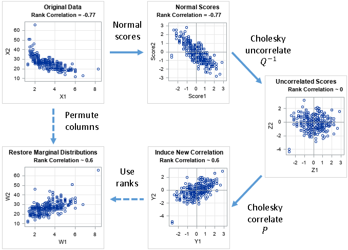
The Iman-Conover transformation is actually a sequence of four transformations. Let X be a data matrix (representing continuous data) and let C be a target rank-correlation matrix. The goal of the Iman-Conover transformation is to permute the elements in the columns of X to create a new data matrix (W) whose rank correlation is close to C. Here are the four steps in the Iman-Conover algorithm:

1. Create normal scores: Compute the van der Waerden normal scores for each column of X. Let S be the matrix of normal scores.
2. Uncorrelate the scores. Let Z be the matrix of uncorrelated scores. Let Q^-1 be the transformation that maps S to Z.
3. Correlated the scores to match the target. Let Y be the correlated scores. Let P be the transformation that maps Z to Y.
4. Reorder the elements in the i_th column of X to match the order of the elements in the i_th column of Y. This ensures that X has the same rank correlation as Y.

The following diagram presents the steps of the Iman-Conover transformation. The original data are in the upper-left graph. The final data are in the lower-left graph. Each transformation is explained in a separate section of this article.

Background information

To understand the Iman-Conover transformation, recall the three mathematical facts that make it possible:

• The van der Waerden scores transform data into new data that are approximately multivariate normal. The new data has the same rank correlation as the original data.
• The Cholesky root of a correlation matrix correlates variables. The inverse of the Cholesky root uncorrelates variables.
• You can change the correlation between variables by permuting the values in the columns of a data matrix. Permuting the values does not change the marginal distributions of the columns.

The purpose of this article is to present the main ideas behind the Iman-Conover transformation. This is not a proof, and almost every sentence should include the word "approximately." For example, when I write, "the data are multivariate normal" or "the data has the specified correlation," you should insert the word "approximately" into those sentences. I also blur the distinction between correlation in the population and sample correlations.

Example data

This example uses the EngineSize and MPG_Highway variables from the Sashelp.Cars data set. These variables are not normally distributed. They have a rank correlation of -0.77. The goal of this example is to permute the values to create new variables that have a rank correlation that is close to a target correlation. This example uses +0.6 as the target correlation, but you could choose any other value in the interval (-1, 1).

The following DATA step creates the data for this example. The graph in the upper-left of the previous diagram shows the negative correlation between these variables:

data Orig;
set sashelp.cars(rename=(EngineSize=X MPG_Highway=Y));
keep X Y;
label X= Y=;
run;

Transformation 1: Create normal scores

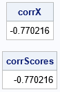
You can compute the van der Waerden scores for each variable. The van der Waerden scores are approximately normal—or at least "more normal" than the original variables. The following SAS/IML statements create the van der Waerden scores as columns of a matrix, S. Because the normalizing transformation is monotonic, the columns of S have the same rank correlation as the original data. The second graph in the previous diagram shows a scatter plot of the columns of S.

proc iml;
varNames = {"X" "Y"};
use Orig; read all var varNames into X; close;
 
/* T1: Create normal scores of each column 
   Columns of S have exactly the same ranks as columns of X.
   ==> Spearman corr is the same    */
N = nrow(X);
S = J(N, ncol(X));
do i = 1 to ncol(X);
   ranks = ranktie(X[,i], "mean");          /* tied ranks */
   S[,i] = quantile("Normal", ranks/(N+1)); /* van der Waerden scores */
end;
/* verify that rank correlation has not changed */
corrScores = corr(S, "Spearman")[2];
print corrX, corrScores;

Transformation 2: Uncorrelate the scores

For many data sets, the van der Waerden scores are approximately multivariate normal. Let C_S be the Pearson correlation matrix of S. Let Q be the Cholesky root of C_S. The inverse of Q is a transformation that removes any correlations among multivariate normal data. Thus, if you use the inverse of Q to transform the scores, you obtain multivariate data that are uncorrelated. The third graph in the previous diagram shows a scatter plot of the columns of Z.

/* T2: use the inverse Cholesky transform of the scores to uncorrelate */
CS = corr(S);        /* correlation of scores */
Q = root(CS);        /* Cholesky root of correlation of scores */
Z = S*inv(Q);        /* uncorrelated MVN data */
corrZ = corr(Z, "Spearman")[2];
print corrZ;

Transformation 3: Correlate the scores

Let C be the target correlation matrix. Let P be its Cholesky root. The matrix P is a transformation that induces the specified correlations in uncorrelated multivariate normal data. Thus, you obtain data, Y, that are multivariate normal with the given Pearson correlation. In most situations, the Spearman rank correlation is close to the Pearson correlation. The fourth graph in the previous diagram shows a scatter plot of the columns of Y.

/* T3: use the Cholesky transform of the target matrix to induce correlation */
/* define the target correlation */
C = {1    0.6,
     0.6 1  };
P = root(C);         /* Cholesky root of target correlation */
Y = Z*P;
corrY = corr(Y, "Spearman")[2];
print corrY;

Transformation 4: Reorder the values in columns of the original matrix

The data matrix Y has the correct correlations, but the Cholesky transformations of the scores have changed the marginal distributions of the scores. But that's okay: Iman and Conover recognized that any two matrices whose columns have the same ranks also have the same rank correlation. Thus, the last step uses the column ranks of Y to reorder the values in the columns of X.

Iman and Conover (1982) assume that the columns of X do not have any duplicate values. Under that assumption, when you use the ranks of each column of Y to permute the columns of X, the rank correlation of Y and X will be the same. (And, of course, you have not changed the marginal distributions of X.) If X has duplicate values (as in this example), then the rank correlations of Y and X will be close, as shown by the following statements:

/* T4: Permute or reorder data in the columns of X to have the same ranks as Y */
W = X; 
do i = 1 to ncol(Y);
   rank = rank(Y[,i]);          /* use ranks as subscripts, so no tied ranks */
   tmp = W[,i]; call sort(tmp); /* sort column by ranks */
   W[,i] = tmp[rank];           /* reorder the column of X by the ranks of Y */
end;
 
corrW = corr(W, "Spearman")[2];
print corrW;

The rank correlation for the matrix W is very close to the target correlation. Furthermore, the columns have the same values as the original data, and therefore the marginal distributions are the same. The lower-left graph in the previous diagram shows a scatter plot of the columns of W.

The effect of tied values

As mentioned previously, the Iman-Conover transformation was designed for continuous variables that do not have any duplicate values. In practice, the Iman-Conover transformation still works well even if there are some duplicate values in the data. For this example, there are 428 observations. However, the first column of X has only 43 unique values and the second column has only 33 unique values. Because the normal scores are created by using the RANKTIE function, the columns of the S matrix also have 43 and 33 unique values, respectively.

Because the Q^-1 matrix is upper triangular, the number of unique values might change for the Z matrix. For these data, the columns of Z and Y have 43 and 194 unique values, respectively. These unique values determine the matrix W, which is why the rank correlation for W is slightly different than the rank correlation for Y in this example. If all data values were unique, then W and Y would have exactly the same rank correlation.

Summary

The Iman-Conover transformation seems magical when you first see it. This article attempts to lift the curtain and reveal the mathematics behind the algorithm. By understanding the geometry of various transformations, you can understand the mathe-magical properties that make the Iman-Conover algorithm an effective tool in multivariate simulation studies.

You can download the complete SAS program that creates all graphs and tables in this article..