Simulating univariate data is relatively easy. Simulating multivariate data is much harder. The main difficulty is to generate variables that have given univariate distributions but also are correlated with each other according to a specified correlation matrix. However, Iman and Conover (1982, "A distribution-free approach to inducing rank correlation among input variables") proposed a transformation that approximately induces a specified correlation among component variables without changing the univariate distribution of the components. (The univariate distributions are called the marginal distributions.) The Iman-Conover transformation is designed to transform continuous variables.

This article defines the Iman-Conover transformation. You can use the transformation to generate a random sample that has (approximately) a given correlation structure and known marginal distributions. The Iman-Conover transformation uses rank correlation, rather than Pearson correlation. In practice, the rank correlation and the Pearson correlation are often close to each other.

This article shows how to use the Iman-Conover transformation. A separate article explains how the Iman-Conover transformation works. The example and SAS program in this article are adapted from Chapter 9 of my book Simulating Data with SAS (Wicklin, 2013).

Create simulated data with known distributions

To use the Iman-Conover transformation, you must specify two things: A set of data and a target correlation matrix. The transformation will induce the specified correlation in the data by rearranging (or permuting) the columns of the data. In other words, the algorithm permutes the columns independently to induce the specified correlation without changing the marginal distributions.

This example generates data with four variables whose marginal distributions are normal, lognormal, exponential, and uniform, respectively. It does not matter whether the original data are correlated or not. For simplicity, generate each variable independently, so the initial correlation matrix is approximately the identity matrix. The following SAS DATA step simulates four variables from the specified distributions. The call to PROC CORR computes the rank correlation of the original data. It also creates a scatter plot matrix that shows the marginal distributions of the variable in the diagonal cells and the bivariate joint distributions in the off-diagonal cells.

%let N = 100; /* sample size */
/* independently simulate variables from known distributions */
data SimIndep;
call streaminit(12345);
do i = 1 to &N;
   Normal    = rand("Normal");
   Lognormal = rand("Lognormal");
   Expon     = rand("Expo");
   Uniform   = rand("Uniform");
   output;
end;
drop i;
run;
 
proc corr data=SimIndep Spearman noprob plots=matrix(hist);
   var Normal Lognormal Expon Uniform;
run;

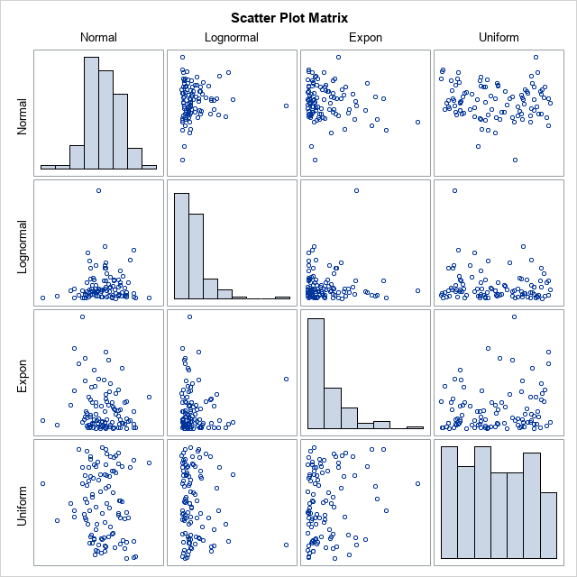
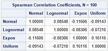
For these simulated data, the table shows that the rank correlation between any pair of variables is small. None of the correlations are statistically different from 0, which you can verify by removing the NOPROB option from the PROC CORR statement.

Implement the Iman-Conover transformation in SAS

The Iman-Conover transformation is actually a sequence of transformations of multivariate data. The following program defines the Iman-Conover transformation as a SAS/IML function. An explanation of the function is provided in a separate article.

/* define a store a SAS/IML function that computes the Iman-Conover transformation */
proc iml;
/* Input: X is a data matrix with k columns
          C is a (k x k) rank correlation matrix
   Output: A matrix W. The i_th column of W is a permutation of the i_th
          columns of X. The rank correlation of W is close to the 
          specified correlation matrix, C.
*/          
start ImanConoverTransform(X, C);
   N = nrow(X);
   S = J(N, ncol(X));
   /* T1: Create normal scores of each column */
   do i = 1 to ncol(X);
      ranks = ranktie(X[,i], "mean");          /* tied ranks */
      S[,i] = quantile("Normal", ranks/(N+1)); /* van der Waerden scores */
   end;
   /* T2: apply two linear transformations to the scores */
   CS = corr(S);        /* correlation of scores */
   Q = root(CS);        /* Cholesky root of correlation of scores */
   P = root(C);         /* Cholesky root of target correlation */
   T = solve(Q,P);      /* same as  T = inv(Q) * P; */
   Y = S*T;             /* transform scores: Y has rank corr close to target C */
 
   /* T3: Permute or reorder data in the columns of X to have the same ranks as Y */
   W = X;
   do i = 1 to ncol(Y);
      rank = rank(Y[,i]);          /* use ranks as subscripts, so no tied ranks */
      tmp = W[,i]; call sort(tmp); /* sort column by ranks */
      W[,i] = tmp[rank];           /* reorder the column of X by the ranks of M */
   end;
   return( W );
finish;
store module=(ImanConoverTransform);  /* store definition for later use */
quit;

Unlike many algorithms in the field of simulation, the Iman-Conover transformation is deterministic. Given a matrix of data (X) and a correlation matrix (C), the function returns the same transformed data every time you call it.

Use the Iman-Conover transformation to simulate correlated data

The following SAS/IML program shows how to use the Iman-Conover transformation to simulate correlated data. There are three steps:

1. Read real or simulated data into a matrix, X. The columns of X define the marginal distributions. For this example, we will use the SimIndep data, which contains four variables whose marginal distributions are normal, lognormal, exponential, and uniform, respectively.
2. Define a "target" correlation matrix. This specifies the rank correlations that you hope to induce. For this example, the target correlation between the Normal and Lognormal variables is 0.75, the target correlation between the Normal and Exponential variables is -0.7, the target correlation between the Normal and Uniform variables is 0, and so forth.
3. Call the ImanConoverTransform function. This returns a new data matrix, W. The i_th column of W is a permutation of the i_th column of X. The permutations are chosen so that the rank correlation of W is close to the specified correlation matrix:

proc iml;
load module=(ImanConoverTransform);  /* load the function definition */
 
/* Step 1: Read in the data */
varNames = {'Normal' 'Lognormal' 'Expon' 'Uniform'};
use SimIndep; read all var varNames into X; close;
 
/* Step 2: specify target rank correlation */
/*    X1    X2    X3    X4                 */
C = { 1.00  0.75 -0.70  0,           /* X1 */
      0.75  1.00 -0.95  0,           /* X2 */
     -0.70 -0.95  1.00 -0.3,         /* X3 */
      0     0    -0.3   1.0};        /* X4 */
 
/* Step 3: Strategically reorder the columns of X. 
           The new ordering has the specified rank corr (approx)
           and preserves the original marginal distributions. */
W = ImanConoverTransform(X, C);
RankCorr = corr(W, "Spearman");
print RankCorr[format=6.3 r=varNames c=varNames];

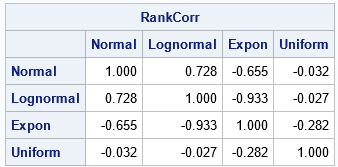
As advertised, the rank correlation of the new data matrix, W, is very close to the specified correlation matrix, C. You can write the data matrix to a SAS data set and use PROC CORR to create a scatter plot matrix that has the marginal histograms on the diagonal:

/* write new data to a SAS data set */
newvarNames = {'newNormal' 'newLognormal' 'newExpon' 'newUniform'};
create SimCorr from W[c=newvarNames];  append from W;  close;
quit;
 
proc corr data=SimCorr Spearman noprob plots=matrix(hist);
   var newNormal newLognormal newExpon newUniform;
run;

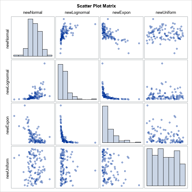
If you compare the diagonal histograms in this graph to the histograms in the previous graph, you will see that they are identical. They have to be identical because each new variable contains exactly the same data values as the original variables.

At the same time, the bivariate scatter plots show how permuting the data has induced the prescribed correlations between the variables. For this example, the newNormal and newLognormal variables have a strong positive rank correlation (0.73). The newNormal and NewExponential variables have a strong negative rank correlation (-0.65). The newNormal and newUniform variables are essentially uncorrelated (-0.03), and so forth.

Summary

The Iman-Conover transformation is a remarkable algorithm that induces a specified correlation structure on a data matrix while preserving the marginal distributions. You start with any data matrix (X) and any target correlation matrix. (The columns of X must represent continuous data.) You apply the Iman-Conover transformation to obtain a new matrix (W). The rank correlation of the new matrix is close to the values you specified. The columns of W have the same values as the columns of X, but the values have been reordered. Thus, the new matrix has the same marginal distributions as the original matrix.

You can download the complete SAS program that defines and uses the Iman-Conover transformation.

In a follow-up article, I explain the geometry or the Iman-Conover transformation and how it works.