This article shows how to use SAS to simulate data that fits a linear regression model that has categorical regressors (also called explanatory or CLASS variables). Simulating data is a useful skill for both researchers and statistical programmers. You can use simulation for answering research questions, but you can also use it generate "fake" (or "synthetic") data for a presentation or blog post when the real data are confidential. I have previously shown how to use SAS to simulate data for a linear model and for a logistic model, but both articles used only continuous regressors in the model.

This discussion and SAS program are based on Chapter 11 in Simulating Data with SAS (Wicklin, 2013, p. 208-209). The main steps in the simulation are as follows. The comments in the SAS DATA program indicate each step:

1. Macro variables are used to define the number of continuous and categorical regressors. Another macro variable is used to specify the number of levels for each categorical variable. This program simulates eight continuous regressors (x1-x8) and four categorical regressors (c1-c4). Each categorical regressor in this simulation has three levels.
2. The continuous regressors are simulated from a normal distribution, but you can use any distribution you want. The categorical levels are 1, 2, and 3, which are generated uniformly at random by using the "Integer" distribution. The discrete "Integer" distribution was introduced in SAS 9.4M5; for older versions of SAS, use the %RandBetween macro as shown in the article "How to generate random integers in SAS." You can also generate the levels non-uniformly by using the "Table" distribution.
3. The response variable, Y, is defined as a linear combination of some explanatory variables. In this simulation, the response depends linearly on the x1 and x8 continuous variables and on the levels of the C1 and C4 categorical variables. Noise is added to the model by using a normally distributed error term.

/* Program based on Simulating Data with SAS, Chapter 11 (Wicklin, 2013, p. 208-209) */
%let N = 10000;                  /* 1a. number of observations in simulated data */
%let numCont =  8;               /* number of continuous explanatory variables */
%let numClass = 4;               /* number of categorical explanatory variables */
%let numLevels = 3;              /* (optional) number of levels for each categorical variable */
 
data SimGLM; 
  call streaminit(12345); 
  /* 1b. Use macros to define arrays of variables */
  array x[&numCont]  x1-x&numCont;   /* continuous variables named x1, x2, x3, ... */
  array c[&numClass] c1-c&numClass;  /* CLASS variables named c1, c2, ... */
  /* the following statement initializes an array that contains the number of levels
     for each CLASS variable. You can hard-code different values such as (2, 3, 3, 2, 5) */
  array numLevels[&numClass] _temporary_ (&numClass * &numLevels);  
 
  do k = 1 to &N;                 /* for each observation ... */
    /* 2. Simulate value for each explanatory variable */ 
    do i = 1 to &numCont;         /* simulate independent continuous variables */
       x[i] = round(rand("Normal"), 0.001);
    end; 
    do i = 1 to &numClass;        /* simulate values 1, 2, ..., &numLevels with equal prob */
       c[i] = rand("Integer", numLevels[i]);        /* the "Integer" distribution requires SAS 9.4M5 */
    end; 
 
    /* 3. Simulate response as a function of certain explanatory variables */
    y = 4 - 3*x[1] - 2*x[&numCont] +                /* define coefficients for continuous effects */
       -3*(c[1]=1) - 4*(c[1]=2) + 5*c[&numClass]    /* define coefficients for categorical effects */
        + rand("Normal", 0, 3);                     /* normal error term */
    output;  
  end;  
  drop i k;
run;     
 
proc glm data=SimGLM;
   class c1-c&numClass;
   model y = x1-x&numCont c1-c&numClass / SS3 solution;
   ods select ModelANOVA ParameterEstimates;
quit;

The ModelANOVA table from PROC GLM (not shown) displays the Type 3 sums of squares and indicates that the significant terms in the model are x1, x8, c1, and c4.

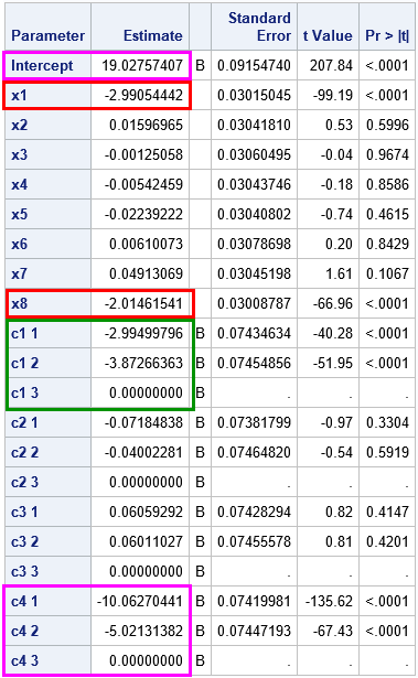
The parameter estimates from PROC GLM are shown to the right. You can see that each categorical variable has three levels, and you can use PROC FREQ to verify that the levels are uniformly distributed. I have highlighted parameter estimates for the significant effects in the model:

• The estimates for the significant continuous effects are highlighted in red. The estimates for the coefficients of x1 and x8 are about -3 and -2, respectively, which are the parameter values that are specified in the simulation.
• The estimates for the levels of the C1 CLASS variable are highlighted in green. They are close to (-3, -4, 0), which are the parameter values that are specified in the simulation.
• The estimates for the Intercept and the C4 CLASS variable are highlighted in magenta. Notice that they seem to differ from the parameters in the simulation. As discussed previously, the simulation and PROC GLM use different parameterizations of the C4 effect. The simulation assigns Intercept = 4. The contribution of the first level of C4 is 5*1, the contribution for the second level is 5*2, and the contribution for the third level is 5*3. As explained in the previous article, the GLM parameterization reparameterizes the C4 effect as (4 + 15) + (5 - 15)*(C4=1) + (10 - 15)*(C4=2). The estimates are very close to these parameter values.

Although this program simulates a linear regression model, you can modify the program and simulate from a generalized linear model such as the logistic model. You just need to compute the linear predictor, eta (η), and then use the link function and the RAND function to generate the response variable, as shown in a previous article about how to simulate data from a logistic model.

In summary, this article shows how to simulate data for a linear regression model in the SAS DATA step when the model includes both categorical and continuous regressors. The program simulates arbitrarily many continuous and categorical variables. You can define a response variable in terms of the explanatory variables and their interactions.