Recently I was asked to explain the result of an ANOVA analysis that I posted to a statistical discussion forum. My program included some simulated data for an ANOVA model and a call to the GLM procedure to estimate the parameters. I was asked why the parameter estimates from PROC GLM did not match the parameter values that were specified in the simulation. The answer is that there are many ways to parameterize the categorical effects in a regression model. SAS regression procedures support many different parameterizations, and each parameterization leads to a different set of parameter estimates for the categorical effects. The GLM procedure uses the so-called GLM-parameterization of classification effects, which sets to zero the coefficient of the last level of a categorical variable. If your simulation specifies a non-zero value for that coefficient, the parameters that PROC GLM estimates are different from the parameters in the simulation.

An example makes this clearer. The following SAS DATA step simulates 300 observations for a categorical variable C with levels 'C1', 'C2', and 'C3' in equal proportions. The simulation creates a response variable, Y, based on the levels of the variable C. The GLM procedure estimates the parameters from the simulated data:

data Have;
call streaminit(1);
do i = 1 to 100;
   do C = 'C1', 'C2', 'C3';
      eps = rand("Normal", 0, 0.2);
      /* In simulation, parameters are Intercept=10, C1=8, C2=6, and C3=1 
         This is NOT the GLM parameterization. */
      Y = 10 + 8*(C='C1') + 6*(C='C2') + 1*(C='C3') + eps;  /* C='C1' is a 0/1 binary variable */
      output;
   end;
end;
keep C Y;
run;
 
proc glm data=Have plots=none;
   class C;
   model Y = C / SS3 solution;
   ods select ParameterEstimates;
quit;

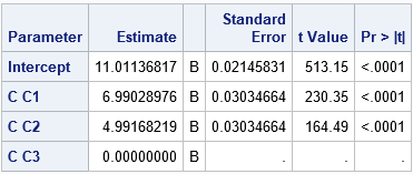
The output from PROC GLM shows that the parameter estimates are very close to the following values: Intercept=11, C1=7, C2=5, and C3=0. Although these are not the parameter values that were specified in the simulation, these estimates make sense if you remember the following:

• When C='C3', the expected response is the sum of the intercept and the 'C3' parameter, which is 10 + 1 = 11. To convert to the GLM parameterization, you need to incorporate the reference level (C3) into the Intercept term. Thus, the Intercept term for the GLM parameterization is 11, not 10.
• In the GLM parameterization, "the parameter estimates of main effects estimate the difference in the effects of each level compared to the last level (in alphabetical order)." To obtain the difference, subtract 1 (the C3 coefficient) from the C1 and C2 coefficients to obtain 7 (8 – 1) and 5 (6 – 1) for the GLM parameters.

In other words, you can use the parameter values in the simulation to convert to the corresponding parameters for the GLM parameterization. In the following DATA step, the Y and Y2 variables contain exactly the same values, even though the formulas look different. The Y2 variable is simulated by using a GLM parameterization of the C variable:

data Have;
call streaminit(1);
refEffect = 1;
do i = 1 to 100;
   do C = 'C1', 'C2', 'C3';
      eps = rand("Normal", 0, 0.2);
      /* In simulation, parameters are Intercept=10, C1=8, C2=6, and C3=1 */
      Y  = 10 + 8*(C='C1') + 6*(C='C2') + 1*(C='C3') + eps;
      /* GLM parameterization for the same response: Intercept=11, C1=7, C2=5, C3=0 */
      Y2 = (10 + refEffect) + (8-refEffect)*(C='C1') + (6-refEffect)*(C='C2') + eps;
      diff = Y - Y2;         /* Diff = 0 when Y=Y2 */
      output;
   end;
end;
keep C Y Y2 diff;
run;
 
proc means data=Have;
   var Y Y2 diff;
run;

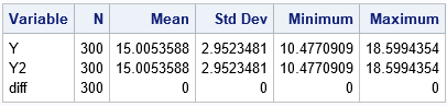
The output from PROC MEANS shows that the Y and Y2 variables are exactly equal. The coefficients for the Y2 variable are 11 (the intercept), 7, 5, and 0, which are the parameter values that are estimated by PROC GLM.

Of course, other parameterizations are possible. For example, you can create the simulation by using other parameterizations such as the EFFECT coding. (The EFFECT coding is the default coding in PROC LOGISTIC.) For the effect coding, parameter estimates of main effects indicate the difference of each level as compared to the average effect over all levels. The following statements show the effect coding for the variable Y3. The values of the Y3 variable are exactly the same as Y and Y2:

avgEffect = 5;   /* average effect for C is (8 + 6 + 1)/3 = 15/3 = 5 */
...
      /* EFFECT parameterization: Intercept=15, C1=3, C2=1, C3=0 */
      Y3 = 10 + avgEffect + (8-avgEffect)*(C='C1') + (6-avgEffect)*(C='C2') + eps;

In summary, when you write a simulation that includes categorical data, there are many equivalent ways to parameterize the categorical effects. When you use a regression procedure to analyze the simulated data, the procedure and simulation might use different parameterizations. If so, the estimates from the procedure might be quite different from the parameters in your simulation. This article demonstrates this fact by using the GLM parameterization and the EFFECT parameterization, which are two commonly used parameterizations in SAS. See the SAS/STAT documentation for additional details about the different parameterizations of classification variables in SAS.