Suppose you want to find observations in multivariate data that are closest to a numerical target value. For example, for the students in the Sashelp.Class data set, you might want to find the students whose (Age, Height, Weight) values are closest to the triplet (13, 62, 100). The way to do this is to compute a distance from each observation to the target. Unfortunately, there are many definitions of distance! Which distance should you use? This article describes and compares a few common distances and shows how to compute them in SAS.

Euclidean and other distances

The two most widely used distances are the Euclidean distance (called the L₂ distance by mathematicians) and the "sum of absolute differences" distance, which is better known as the L₁ distance or occasionally the taxicab distance. In one dimension, these distances are equal. However, when you have multiple coordinates, the distances are different. The Euclidean and L₁ distances between (x1, x2, ..., xn) and a target vector (t1, t2, ..., tn) are defined as follows:
L₁ distance: |x1-t1| + |x2-t2| + ... + |xn-tn|
Euclidean distance: sqrt( (x1-t1)² + (x2-t2)² + ... + (xn-tn)² )

Both of these distances are supported in the SAS DATA step. You can use the EUCLID function to compute Euclidean distance and use the SUMABS function to compute the L₁ distance. For example, the following DATA step computes the distance from each observation to the target value (Age, Height, Weight) = (13, 62, 100):

data Closest;
/* target (Age, Height, Weight) = (13, 62, 100) */
set Sashelp.Class;
EuclidDist = euclid(Age-13, Height-62, Weight-100);
L1Dist     = sumabs(Age-13, Height-62, Weight-100);
run;
 
/* sort by Euclidean distance */
proc sort data=Closest out=Euclid; by EuclidDist; run;
 
/* plot the distances for each observation */
title "Distance to Target Values";
proc sgplot data=Euclid;
   series x=Name y=EuclidDist / curvelabel="Euclidean";  *datalabel=Weight;
   series x=Name y=L1Dist     / curvelabel="L1";         *datalabel=Weight;
   yaxis grid label="Distance";
   xaxis grid discreteorder=data;
run;

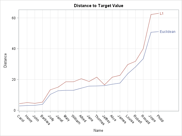
The graph shows the Euclidean and L₁ distances from each student's data to the target value. The X axis is ordered by the Euclidean distance from each observation to the target value. If you add the DATALABEL=Weight or DATALABEL=Height options to the SERIES statements, you can see that the students who appear near the left side of the X axis have heights and weights that are close to the target values (Height, Weight) = (62, 100). The students who appear to the right are much taller/heavier or shorter/lighter than the target values. In particular, Joyce is the smallest student and Philip is the largest.

If you order the students by their L₁ distances, you will obtain a different ordering. For example, in an L₁ ranking, John and Henry would switch positions and Jeffery would be ranked 7th instead of 12th.

Distances that account for scale

There is a problem with the computations in the previous section: the variables are measured in different units, but the computations do not account for these differences. In particular, Age is an important factor in the distance computations because all student ages are within three years of the target age. In contrast, the heaviest student (Phillip) is 88 pounds more than the target weight.

The distance formula needs to account for amount of variation within each variable. If you run PROC MEANS on the data, you will discover that the standard deviation of the Age variable is about 1.5, whereas the standard deviations for the Height and Weight variables are about 5.1 and 22.8, respectively. It follows that one year should be treated as a substantial difference, whereas one pound of weight should be treated as a small difference.

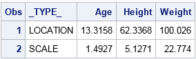
A way to correct for differences among the scales of variables is to standardize the variables. In SAS, you can use PROC STDIZE to standardize the variables in a variety of ways. By default, the procedure centers each variable by subtracting the sample mean; it scales by dividing by the standard deviations. The following procedure all also writes the mean and standard deviations to a data set, which is displayed by using PROC PRINT:

proc stdize data=Sashelp.Class out=StdClass outstat=StdIn method=STD;
   var Age Height Weight;
run;
 
proc print data=StdIn(obs=2);
run;

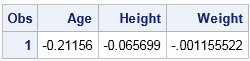
Notice that target value is not part of the standardization! Only the data are used. However, you must convert the target value to the new coordinates before you can compute the standardized distances. You can standardize the target value by using the METHOD=IN option in PROC STDIZE to tell the procedure to transform the target value by using the location and scale values in the StdIn data set, as follows:

data Target;
   Age=13; Height=62; Weight=100;
run;
 
proc stdize data=Target out=StdTarget method=in(StdIn);
   var Age Height Weight;
run;
 
proc print data=StdTarget; run;

The data and the target values are now in standardized coordinates. You can therefore repeat the earlier DATA step and compute the Euclidean and L₁ distances in the new coordinates. The graph of the standardized distances are shown below:

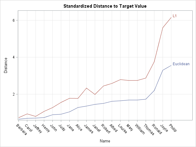
In the standardized coordinates "one unit" corresponds to one standard deviation from the mean in each variable. Thus Age is measured in units of 1.5 years, Height in units of 5.1 inches, and Weight in units of 22.8 pounds. Notice that some of the students have changed positions. Carol is still very similar to the target value, but Jeffrey is now more similar to the target value than previously thought. The smallest student (Joyce) and largest student (Philip) are still dissimilar (very distant) from the target.

Distances that account for correlation

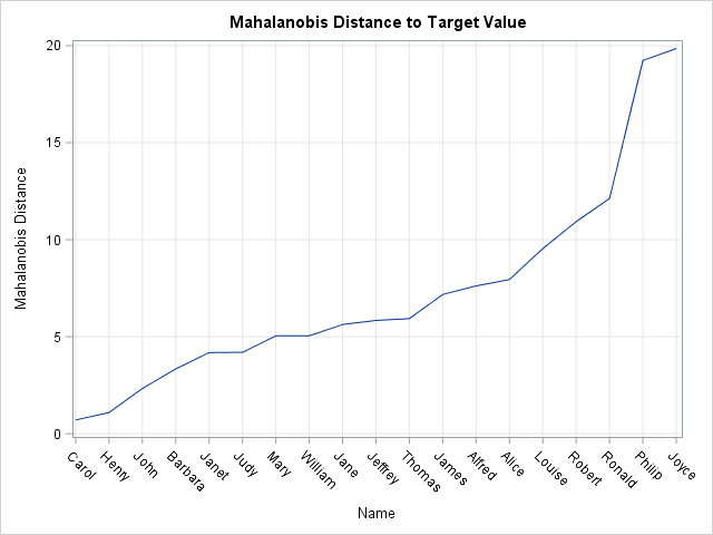
In the previous section, different scales in the data are handled by using distances in a standardized coordinate system. This is an improvement over the unstandardized computations. However, there is one more commonly used distance computation, called the Mahalanobis distance. The Mahalanobis distance is similar to the standardized L₂ distance but also accounts for correlations between the variables. I have previously discussed the meaning of Mahalanobis distance and have described how you can use the inverse Cholesky decomposition to uncorrelate variables. I won't repeat the arguments, but the following graph displays the Mahalanobis distance between each observation and the target value. Some students are in a different order than they were for the standardized distances:

If you would like to examine or modify any of my computations, you can download the SAS program that computes the various distances.

In summary, there are several reasonable definitions of distance between multivariate observations. The simplest is the raw Euclidean distance, which is appropriate when all variables are measured on the same scale. The next simplest is the standardized distance, which is appropriate if the scales of the variables are vastly different and the variables are uncorrelated. The third is the Mahalanobis distance, which becomes important if you want to measure distances in a way that accounts for correlation between variables.

For other articles about Mahalanobis distance or distance computations in SAS, see:

• "How to compute Mahalanobis distance in SAS"
• "How to compute the distance between observations in SAS"
• "Distances between observations in two groups"