I recently blogged about Mahalanobis distance and what it means geometrically. I also previously showed how Mahalanobis distance can be used to compute outliers in multivariate data. But how do you compute Mahalanobis distance in SAS?
Computing Mahalanobis distance with built-in SAS procedures and functions
There are several ways to compute the Mahalanobis distances between observations and the sample mean. One way is to compute the leverage statistic by using a regression procedure, and then using a mathematical relationship between the leverage and the Mahalanobis distance. To find the Mahalanobis distance between pairs of points, you can use principal component analysis and the DISTANCE procedure. And, as mentioned in a previous blog, the MCD routine in SAS/IML software provides the classical Mahalanobis distance for a data matrix.
UPDATE (Sept 2012): As of SAS/IML 12.1, which shipped in August 2012 as part of SAS 9.3m2, the MAHALANOBIS function is distributed as part of SAS/IML software. You do not need to read the following sections unless you want to understand how the MAHALANOBIS function works.
Writing a Mahalanobis distance function
The previous methods all have a disadvantage: they provide the Mahalanobis distance as a consequence of computing something else (regression, principal components, or MCD). However, if your goal is to compute the Mahalanobis distance, it is more efficient to call a function that is designed for that purpose. You can use the SAS/IML language to write such a function.
Rather than just present a Mahalanobis distance function in its final form, I'm going to describe three functions: the naive "first attempt" function, a more efficient alternative, and a final function that is both efficient and can be used in a variety of situations.
A first attempt: Implement the mathematical formula
One of the advantages of the SAS/IML language is that it enables you to use a natural syntax to implement mathematical formulas that appear in textbooks and journal articles. Given an observation x from a multivariate normal distribution with mean μ and covariance matrix Σ, the squared Mahalanobis distance from x to μ is given by the formula d2 = (x - μ)T Σ -1 (x - μ). You can use this definition to define a function that returns the Mahalanobis distance for a row vector x, given a center vector (usually μ or an estimate of μ) and a covariance matrix:
proc iml;
/* simplest approach: x and center are row vectors */
start mahal1(x, center, cov);
   y = (x - center)`; /* col vector */
   d2 = y` * inv(cov) * y; /* explicit inverse. Not optimal */
   return (sqrt(d2));
finish;

x = {1 0};  /* test it */
center = {1 1};
cov = {9 1,
       1 1};
md1 = mahal1(x, center, cov);
print md1; |

This naive implementation computes the Mahalanobis distance, but it suffers from the following problems:
- The function uses the SAS/IML INV function to compute an explicit inverse matrix. However, it is rarely necessary to compute an explicit matrix inverse. (See also the comments to John D. Cook's article "Don’t invert that matrix.") Explicit computations are less stable numerically and are less efficient than matrix factorization methods.
- The function as written takes a single observation for x and returns a single distance. The function should be generalized so that you can pass in a matrix for x, where each row of the matrix is an observation. The function should return a vector of distances, one for each row of x.
A second attempt: More efficient and more general
Instead of computing the explicit inverse for the given covariance matrix, you can use the Cholesky decomposition (found by the ROOT function in SAS/IML software) followed by solving a linear system by using the TRISOLV function, as described in my article on the Cholesky transformation. You can compute the distance for multiple rows of x by using a DO loop. A second version of the Mahalanobis function follows:
/* (1) Use ROOT and TRISOLV instead of INV to solve linear system
(2) Let x be a matrix. Compute distances from row x[i,] to center. */
start mahal2(x, center, cov);
/* x[i,] and center are row vectors */
n = nrow(x);
d2 = j(n,1); /* allocate vector for distances */
U = root(cov);
/* Want d2 = v * inv(cov) * v` = v * w where cov*w = v`
==> (U`U)*w = v` Cholesky decomp of cov
==> First solve U` z = v` for z,
then solve U w = z for w */
y = x - center;
do i = 1 to n; /* using the DO loop is not optimal */
v = y[i,]; /* get i_th centered row */
z = trisolv(2, U, v`); /* solve linear system */
w = trisolv(1, U, z);
d2[i,] = v * w; /* dot product of vectors */
end;
return (sqrt(d2));
finish;
x = {1 0, /* test it: x has more than one row */
0 1,
-1 0,
0 -1};
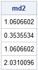
md2 = mahal2(x, center, cov);
print md2; |
This is not a bad algorithm, but it can be improved. Currently it computes distances from a bunch of points (the rows of x) to a single point (passed in as center). However, if you want to compute pairwise distances between two sets of points, you would need to call this function multiple times, and each function call would perform the same Cholesky decomposition. An improvement is to allow the center argument to also be a matrix, and have the function return a matrix of distances, where the (i,j)th distance is the Mahalanobis distance between the ith row of x and the jth row of center.
There are two tricks that you can use to make the new implementation of the Mahalanobis distance function as efficient as possible:
- The TRISOLV function enables you to solve multiple linear systems in a single call by passing in multiple "right-hand sides." Consequently, you don't actually need the DO loop in the previous section to loop over the rows of x.
- It turns out that the squared distance can be written in terms of the diagonal elements of a certain matrix product. In a previous blog, I showed an efficient shortcut for computing the diagonal elements of a matrix product without actually forming the product.
/* 3) Enable pairwise Mahalanobis distances by allowing 2nd arg to be a matrix.
4) Solve linear system for many right-hand sides at once */
start mahalanobis(x, center, cov);
/* x[i,] and center[i,] are row vectors */
n = nrow(x);
m = nrow(center);
d2 = j(n,m); /* return matrix of pairwise Mahalanobis distances */
U = root(cov); /* solve for Cholesky root once */
do k = 1 to m; /* for each row of the center matrix */
v = x - center[k,]; /* v is matrix of right-hand sides */
z = trisolv(2, U, v`); /* solve n linear systems in one call */
w = trisolv(1, U, z);
/* Trick: vecdiag(A*B) = (A#B`)[,+] without computing product */
d2[,k] = (v # w`)[,+]; /* shortcut: diagonal of matrix product */
end;
return (sqrt(d2));
finish;
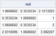
y = {1 1, 0 0, 1 2}; /* x and y are BOTH matrices */
md = mahalanobis(x, y, cov); /* compute pairwise distances between x and y */
print md; |
In summary, you can write a function in the SAS/IML language to compute the Mahalanobis distance in SAS. This single function enables you to compute the Mahalanobis distance for three common situations:
- from each observation to the mean: md = mahalanobis(x, mean(x), cov(x))
- from each observation to a specific observation: md = mahalanobis(x, MyObs, cov(x))
- from each observation to all other observations (all possible pairs): p=x; md = mahalanobis(x, p, cov(x))

20 Comments
For the mahalnobis example, would it be possible to provide an example of what the dataset should look like, please? Thank you
To use this code with a SAS data set, the p variables should be in p columns of the data set.
For example:
data mydata;
input x1-x10;
datalines;
...data here...
;
In PROC IML you can then say:
use mydata;
read all var _NUM_ into X; /* or specify names of vars */
center = mean(X);
cov = cov(X);
md = mahalanobis(x, center, cov);
I have 8 variables: x1-x8
I want to compute the Mahalanobis Distance from a reference point of 7 for each of the variables.
How do I modify the above code to perform this?
You can ask SAS-related questions at the SAS Support Communities. See the links in the right-hand sidebar.
Pingback: The curse of dimensionality: How to define outliers in high-dimensional data? - The DO Loop
Pingback: Compute the multivariate normal denstity in SAS - The DO Loop
Hey, I want to know if sumone can help me on how to calculate the covariance between two matrices X and Y in proc iml sas. For example
X = {1 2, 3 4}
Y = {1 2 , 5 6}
cov(X,Y)
Thank you
You need to explain what you mean. What is cov(X,Y) for your example? Are you asking for the matrix of pairwise covariances for each distinct pair of variables X_i and Y_j (which results in a 2x2 matrix) or some kind of 4x4 block covariance matrix?
Good day, I have actually obtain the correct answer after looking through several code you have posted around the web. Thanks I lot.
/*Calculate the Covariance*/
start covar(x,y);
n_sim = max(Ncol(x),Nrow(x));
ans = (sum(x#y) - (sum(x)*sum(y))/n_sim)/n_sim;
return(ans);
finish;
This isn't any covariance that I am familiar with. It returns a scalar, rather than a matrix. Furthermore,
if X=Y=Identity(n) [the nxn identity matrix] the "Ju Covariance" of an identity matrix with itself is 0. I suggest that you ask help from a local statistician at your workplace or school.
Pingback: SAS blogger on statistics, big data and simplicity - SAS Voices
Hi!
I really need your help. Say I have multiple-group data (group=4, number of variables=4, where each group has 5 observation). I am using MD formula [D^2=(x1bar-x2bar)'S(inverse)(x1bar-x2bar)] for calculation. My intention was; I wanted to rank the variables based on the D^2 (as above formula). I have calculated the D^2, and the table of D^2 that I got describes the distance for groups pairs. The question is how can I find the D^2 for each variable so that I can rank the variables? Please help me:) Thank you very much.
You can ask general statistics questions at the SAS Support Community.
Pingback: How to compute the distance between observations in SAS - The DO Loop
Dr. Wicklin. Thank you for your work, which I have found to be an exceptional resource.
A practical question: Would you care to comment on the possibility of computing the MD or MD^2 in the presence of a covariance matrix (and also invereted covariance matrix) which is not positive definite? Some MD^2's could be negative as a result. Assuming the original covariance matrix did not become non positive definite because of sampling problems (id est, those negative values in the covariance matrix have true meaning), is it reasonable to attempt an interpretation of a negative MD^2, or the magnitude of negativity? Should just those negative MD^2 points be discounted, or are ALL results coming from a non positive definite covaraince matrix invalid to begin with?
I think it depends on your application. Mathematically, a non-PD matrix does not generate a metric and the resulting formula does not satisfy the axioms of a distance. At the same time, in factor analysis, you often estimate a matrix that might not be PD so this case does arise in practice. In that case the estimate of the "Total variance" can be greater than 1. See the doc for PROC FACTOR or this page: http://support.sas.com/documentation/cdl/en/imlsug/63546/HTML/default/viewer.htm#imlsug_ugmultfactor_sect001.htm
I am not an expert on factor analysis, but it seems to me that the problem is that the ESTIMATES are not PD and so statisticians try to jump through loops to make sense of something that is (I think) inherently nonsensical.
Thank you for taking the time to think aobut my question. You confirm my own instinct, it depends on the application.
The subject comes up in finance, for example with the application of mean-variance portfolio theory in constructing an "efficient frontier". See, for example:
http://epublications.bond.edu.au/cgi/viewcontent.cgi?article=1078&context=ejsie
The same portfolio covariance matrix in that application, containing some negative price-change (return) covariance (which does occur in practice, and often results in a non PD matrix) leads to my question with respect to the MD^2.
Dear Dr Rick Wicklin,
Te following R-code can produce the distribution function of the multivariate normal distribution for arbitrary limits and correlation matrices. How can I do the same in SAS please. Your help is greatly appreciated.
pmvnorm(lower=-Inf, upper=Inf, mean=rep(0, length(lower)),
corr=NULL, sigma=NULL, maxpts = 25000, abseps = 0.001,
releps = 0)
Arguments
lower the vector of lower limits of length n.
upper the vector of upper limits of length n.
mean the mean vector of length n.
corr the correlation matrix of dimension n.
sigma the covariance matrix of dimension n. Either corr or sigma can be specified. If sigma is given, the problem is standardized. If neither corr nor sigma is given, the identity matrix is used for sigma.
SAS provides the PROBBNRM function for computing the CDF of a bivariate normal distribution, but does not provide a built-in function that computes the CDF for other multivariate probability distributions. You can use Monte Carlo estimates to estimate the probabilities, but the MC method becomes computationally expensive for high dimensions (five or more).
Your swift response is greatly appreciated. Many thanks Dr Wicklin.