Last week I showed how to find the nearest neighbors for a set of d-dimensional points. A SAS user wrote to ask whether something similar could be done when you have two distinct groups of points and you want to find the elements in the second group that are closest to each element in the first group.

The answer is yes, and this problem occurs frequently in applications. Typically the first group contains the locations of randomly placed individuals and the second contains the locations of resources. For each individual, you want to find the closest resources. Examples include:

• The first group contains the positions of houses. The second group contains the locations of stores. A retailer might want to identify the stores that are closest to customers, so that shipping costs are minimized.
• The first group contains the locations of vehicle accidents on a highway. The second group contains the locations of hospitals who can treat the injured victims.
• The first group contains the location of cell phone users. The second group contains the locations of cell towers.

This article solves the problem in a straightforward way: compute all the pairwise distances between the points in each group. Distances within groups are not needed, so they are not computed.

Compute the pairwise distances between points

I previously showed how to compute the pairwise distance between points in different sets. Let S be a set of n d-dimensional points and let R be another set of m points. The PairwiseDist function in SAS/IML (shown below) returns an n x m matrix, D, of distances such that D[i,j] is the distance from the i_th point in S to the j_th point in R. The PairwiseNearestNbr function is the same algorithm that was used to find nearest neighbors, so I will not re-explain how the function works. Suffice it to say that it returns two matrices: a matrix of row numbers and a matrix or distances. If you have access to In SAS/IML 14.3 (released as part of SAS 9.4M5), the DISTANCE function in PROC IML can compute pairwise distances, as shown in the previous article.

proc iml;
/* https://blogs.sas.com/content/iml/2013/03/27/compute-distance.html */
/* compute Euclidean distance between points in S and points in R.
   S is an n x d matrix, where each row is a point in d dimensions.
   R is an m x d matrix.
   The function returns the n x m matrix of distances, D, such that
   D[i,j] is the distance between S[i,] and R[j,].
*/
start PairwiseDist(S, R);  /* In SAS/IML 14.3, use the built-in DISTANCE(S,R) function */
   if ncol(S)^=ncol(R) then return (.);       /* different dimensions */
   n = nrow(S);  m = nrow(R);
   idx = T(repeat(1:n, m));                   /* index matrix for S   */
   jdx = shape(repeat(1:m, n), n);            /* index matrix for R   */
   diff = S[idx,] - R[jdx,];
   return( shape( sqrt(diff[,##]), n ) );     /* sqrt(sum of squares) */
finish;
 
/* Compute indices (row numbers) of k nearest neighbors.
   INPUT:  S    an (n x d) data matrix
           R    an (m x d) matrix of reference points
           k    specifies the number of nearest neighbors (k>=1) 
   OUTPUT: idx  an (n x k) matrix of row numbers. idx[,j] contains the
                row numbers (in R) of the j_th closest elements to S
           dist an (n x k) matrix. dist[,j] contains the distances
                between S and the j_th closest elements in R
*/
start PairwiseNearestNbr(idx, dist, S, R, k=1);
   n = nrow(S);
   idx = j(n, k, .);
   dist = j(n, k, .);
   D = PairwiseDist(S, R);      /* n x m. Use DISTANCE(S, R) in SAS/IML 14.3 */
   do j = 1 to k;
      dist[,j] = D[ ,><];       /* smallest distance in each row */
      idx[,j] = D[ ,>:<];       /* column of smallest distance in each row */
      if j < k then do;         /* prepare for next closest neighbors */
         ndx = sub2ndx(dimension(D), T(1:n)||idx[,j]);
         D[ndx] = .;            /* set elements to missing */
      end;      
   end;
finish;

An example of finding nearest points

To illustrate how you can use these functions, consider two sets S and R. The set R is the set of resources locations (stores, hospitals, towers,...). For this example, R contains four points that are the vertices of a square of side length 2 centered at the origin. For each point in S, the following SAS/IML statements compute the closest vertex in R and the second-closest-vertex in R:

/* R = vertices of a square */
R = {-1 -1,      /* Pt 1: lower left corner   */
      1 -1,      /* Pt 2: lower right corner  */
      1  1,      /* Pt 3: upper  right corner */
     -1  1};     /* Pt 4: upper left corner   */
S = {-0.3 -0.2,  /* points inside square */
      0.9  0.6,
     -0.5  0.8};
k = 2;          /* find nearest and second nearest points */
run PairwiseNearestNbr(idx, dist, S, R, k);
print idx[c={"Closest" "2nd Closest"} r=("S1":"S3")];

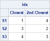
The first column in the table shows the indices (row numbers) of the vertices that are nearest to each point of S. The second column shows the second-closest vertices. For example, Pt 1 (the lowest left corner) is the nearest vertex to the first row of S, and Pt 4 (upper left corner) is the second nearest. In a similar way, Pt 3 is the closest vertex to the second row of S, and Pt 4 is the closest vertex to the third row of S.

The PairwiseNearestNbr module also returns the dist matrix, which contains the corresponding distances. The i_th row of dist contains the distances from the i_th row of S to the two closest vertices.

Coloring points by the closest reference point

In a similar way, you can generate random points in the square and color each point in a scatter plot according to the nearest point in the reference set. The ODS GRAPHICS statement with ATTRPRIORITY=NONE forces the ODS style to cycle though colors and symbols.

ods graphics / attrpriority=NONE width=400px height=400px; /* cycle symbols and colors */
/* Generate 500 random points in square [-1,1] x [-1,1] */
call randseed(12345);
S = R // randfun({500 2}, "Uniform", -1, 1);
k = 2;
 
run PairwiseNearestNbr(idx, dist, S, R, k);
Corner = idx[,1];                            /* index of nearest vertex */
title "Points colored by nearest corner";
call scatter(S[,1], S[,2]) group=Corner grid={x y} procopt="aspect=1";

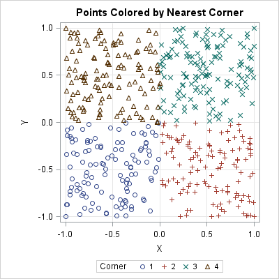
The scatter plot shows what you already knew: points in the first quadrant (green Xs) are closest to the vertex at (1,1). Points in the second quadrant (brown triangles) are closest to the vertex at (-1, 1), and so forth. Any points that are equidistant from two or more vertices (such as the origin) are assigned one of the colors arbitrarily. The points were sorted (not shown) so that the order in the legend agrees with the order of the points in R.

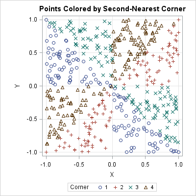
The call to the PairwiseNearestNbr subroutine used k=2, which requests the closest and the second closest points. The second-closest indices are located in the second column of the idx matrix. If you change the title and set Corner = idx[,2], you can create a scatter plot in which each point is colored by the second-closest vertex. That coloration is shown in the scatter plot below. See if you can understand why each marker in the following scatter plot is colored the way it is. For example, for the point in the first quadrant, their second-closest vertex is either the second vertex (1, -1) or the fourth vertex (-1, 1).

In summary, last week I showed how you can find the nearest neighbors among a single set of observations. This article solves a similar problem in which observations are split into two different groups. The functions in this article find the nearest observation in a "reference" or "resource" group for each observation in another group.

I'll conclude by mentioning that you can use these computations to compute the nearest distance between two groups of observations. Simply use k=1 and take the minimum distance that is computed by the PairwiseNearestNbr subroutine. This gives the smallest distance between any point in the first group and any point in the second group.