Visualize a design matrix

Most SAS regression procedures support a CLASS statement which internally generates dummy variables for categorical variables. I have previously described what dummy variables are and how are they used. I have also written about how to create design matrices that contain dummy variables in SAS, and in particular how to use different parameterizations: GLM, reference, effect, and so forth.

It occurs to me that you can visualize the structure of a design matrix by using the same technique (heat maps) that I used to visualize missing value structures. In a design matrix, each categorical variable is replaced by several dummy variables. However, there are multiple parameterizations or encodings that result in different design matrices.

Heat maps of design matrices: GLM parameterization

Heat maps require several pixels for each row and column of the design matrix, so they are limited to small or moderate sized data. The following SAS DATA step extracts the first 150 observations from the Sashelp.Heart data set and renames some variables. It also adds a fake response variable because the regression procedures that generate design matrices (GLMMOD, LOGISTIC, GLMSELECT, TRANSREG, and GLIMMIX) require a response variable even though the goal is to create a design matrix for the explanatory variables. In the following statements, the OUTDESIGN option of the GLMSELECT procedure generates the design matrix. The matrix is then read into PROC IML where the HEATMAPDISC subroutine creates a discrete heat map.

/* add fake response variable; for convenience, shorten variable names */
data Temp / view=Temp;
   set Sashelp.heart(obs=150
                keep=BP_Status Chol_Status Smoking_Status Weight_Status);
   rename BP_Status=BP Chol_Status=Chol 
          Smoking_Status=Smoking Weight_Status=Weight;
   FakeY = 0;
run;
 
ods exclude all;  /* use OUTDESIGN= option to write the design matrix to a data set */
proc glmselect data=Temp outdesign(fullmodel)=Design(drop=FakeY);
   class BP Chol Smoking Weight / param=GLM;
   model FakeY = BP Chol Smoking Weight;
run;
ods exclude none;
 
ods graphics / width=500px height=800px;
proc iml;  /* use HEATMAPDISC call to create heat map of design */
use Design;  read all var _NUM_ into X[c=varNames];  close;
run HeatmapDisc(X) title="GLM Design Matrix"
     xvalues=varNames displayoutlines=0 colorramp={"White" "Black"};
QUIT;

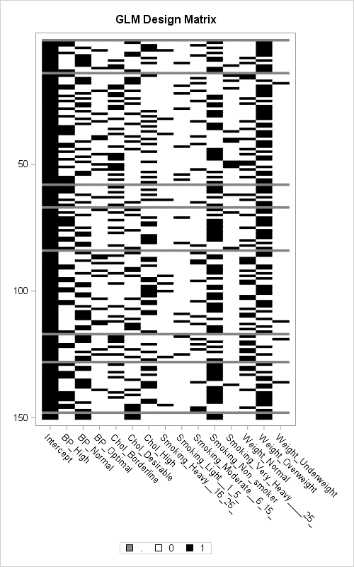
Design matrix for the GLM parameterization in SAS

Click on the heat map to enlarge it. Each row of the design matrix indicates a patient in a research study. If any explanatory variable has a missing value, the corresponding row of the design matrix is missing (shown as gray). In the design matrix for the GLM parameterization, a categorical variable with k levels is represented by k columns. The black and white heat map shows the structure of the design matrix. Black indicates a 1 and white indicates a 0. In particular:

This first column is all black, which indicates the intercept column.
Columns 2-4 represent the BP variable. For each row has one black rectangle in one of those columns. You can see that there are few black squares in column 4, which indicates that few patients in the study have optimal cholesterol.
In a similar way, you can see that there are many nonsmokers (column 11) in the study. There are also many overweight patients (column 14) and few underweight patients (column 15).

The GLM parameterization is called a "singular parameterization" because each it contains redundant columns. For example, the BP_Optimal column is redundant because that column contains a 1 only when the BP_High and BP_Normal columns are both 0. Similarly, if either the BP_High or the BP_Normal columns is 1, then BP_Optimal is automatically 0. The next section removes the redundant columns.

Heat maps of design matrices: Reference parameterization

There is a binary design matrix that contains only the independent columns of the GLM design matrix. It is called a reference parameterization and you can generate it by using PARAM=REF in the CLASS statement, as follows:

ods exclude all;  /* use OUTDESIGN= option to write the design matrix to a data set */
proc glmselect data=Temp outdesign(fullmodel)=Design(drop=FakeY);
   class BP Chol Smoking Weight / param=REF;
   model FakeY = BP Chol Smoking Weight;
run;
ods exclude none;

Design matrix for the REFERENCE parameterization in SAS

Again, you can use the HEATMAPDISC call in PROC IML to create the heat map. The matrix is similar, but categorical variables that have k levels are replaced by k–1 dummy variables. Because the reference level was not specified in the CLASS statement, the last level of each category is used as the reference level. Thus the REFERENCE design matrix is similar to the GLM design, but that the last column for each categorical variable has been dropped. For example, there are columns for BP_High and BP_Normal, but no column for BP_Optimal.

Nonbinary designs: The EFFECT parameterization

The previous design matrices were binary 0/1 matrices. The EFFECT parameterization, which is the default parameterization for PROC LOGISTIC, creates a nonbinary design matrix. In the EFFECT parameterization, the reference level is represented by using a -1 and a nonreference level is represented by 1. Thus there are three values in the design matrix.

If you do not specify the reference levels, the last level for each categorical variable is used, just as for the REFERENCE parameterization. The following statements generate an EFFECT design matrix and use the REF= suboption to specify the reference level. Again, you can use the HEATMAPDISC subroutine to display a heat map for the design. For this visualization, light blue is used to indicate -1, white for 0, and black for 1.

ods exclude all;  /* use OUTDESIGN= option to write the design matrix to a data set */
proc glmselect data=Temp outdesign(fullmodel)=Design(drop=FakeY);
   class BP(ref='Normal') Chol(ref='Desirable') 
         Smoking(ref='Non-smoker') Weight(ref='Normal') / param=EFFECT;
   model FakeY = BP Chol Smoking Weight;
run;
ods exclude none;
 
proc iml;  /* use HEATMAPDISC call to create heat map of design */
use Design; read all var _NUM_ into X[c=varNames]; close;
run HeatmapDisc(X) title="Effect Design Matrix"
     xvalues=varNames displayoutlines=0 colorramp={"LightBlue" "White" "Black"};
QUIT;

Design matrix for the EFFECT parameterization in SAS

In the adjacent graph, blue indicates that the value for the patient was the reference category. White and black indicates that the value for the patient was a nonreference category, and the black rectangle appears in the column that indicates the value of the nonreference category. For me, this design matrix takes some practice to "read." For example, compared to the GLM matrix, it is harder to determine the most frequent levels for a categorical variable.

Heat maps in Base SAS

In the example, I have used the HEATMAPDISC subroutine in SAS/IML to visualize the design matrices. But you can also create heat maps in Base SAS.

If you have SAS 9.4m3, you can use the HEATMAPPARM statement in PROC SGPLOT to create these heat maps. First you have to convert the data from wide form to long form, which you can do by using the following DATA step:

/* convert from wide (matrix) to long (row, col, value)*/
data Long;
set Design;
array dummy[*] _NUMERIC_;
do varNum = 1 to dim(dummy);
   rowNum = _N_;
   value = dummy[varNum];
   output;
end;
keep varNum rowNum value;
run;
 
proc sgplot data=Long;
/* the observation values are in the order {1, 0, -1}; use STYLEATTRIBS to set colors */
styleattrs  DATACOLORS=(Black White LightBlue);
heatmapparm x=varNum y=rowNum colorgroup=value / showxbins discretex;
xaxis type=discrete; /* values=(1 to 11)  valuesdisplay=("A" "B" ... "J" "K"); */
yaxis reverse;
run;

The heat map is similar to the one in the previous section, except that the columns are labeled 1, 2, 3, and so forth. If you want the columns to contain the variable names, use the VALUESDISPLAY= option, as shown in the comments.

If you are running an earlier version of SAS, you will need to use the Graph Template Language (GTL) to create a template for the discrete heat maps.

In summary, you can use the OUTDESIGN= option in PROC GLMSELECT to create design matrices that use dummy variables to encode classification variables. If you have SAS/IML, you can use the HEATMAPDISC subroutine to visualize the design matrix. Otherwise, you can use the HEATMAPPARM statement in PROC SGPLOT (SAS 9.4m3) or the GTL to create the heat maps. The visualization is useful for teaching and understanding the different parameterizations schemes for classification variables.

Blogs