When the SAS Global Forum 2020 conference was cancelled by the global COVID-19 pandemic, I felt sorry for the customers and colleagues who had spent months preparing their presentations. One presentation I especially wanted to attend was by Bucky Ransdell and Randy Tobias: "Introducing PROC SIMSYSTEM for Systematic Nonnormal Simulation". Their paper introduces a new SAS Viya procedure which simplifies running simulation studies and enables you to systematically vary the skewness and kurtosis of univariate distributions.

In my book, Simulating Data with SAS (Wicklin, 2013), I wrote more than 20 pages in Chapter 16 that explains how to write SAS code to perform the computations that PROC SIMSYSTEM can perform with a much simpler (and shorter!) syntax. This article explains the purpose of PROC SIMSYSTEM and shows how to use it for an introductory example. PROC SIMSYSTEM is available in SAS Visual Statistics in SAS Viya; it is not available in SAS 9.4.

Flexible distributions

The search for a flexible distribution that can model almost any data distribution is the Holy Grail of distributional modeling. The goal is to find a family of distributions that can model any univariate data distribution. The distributions in the family must be easy to fit and easy to simulate from. The SIMSYSTEM procedure implements the techniques of Pearson (circa 1895) and Johnson (1949) and provides an easy interface for generating random samples from the Pearson or Johnson system of distributions. Both systems rely on moment matching to fit the parameters in the models. That is, you specify the moments (mean, standard deviation, skewness, and kurtosis) of a univariate distribution, and the procedure selects a distribution and parameter values for which the distribution has the specified moments. In addition, you can ask for random samples from that distribution, which you can use in a Monte Carlo simulation.

This article demonstrates the simple task of specifying moments and generating samples from a distribution in the Johnson system that has those moments. This enables you to investigate how an estimator or statistical test perform on samples whose skewness and kurtosis vary in a systematic way.

Using the moments of a bounded distribution

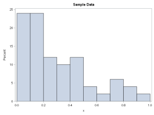
Suppose you have a data sample that is bounded in the interval [0, 1], such as shown to the right. You could model the data by using a Beta distribution. Alternatively, you can use the Johnson SB distribution. PROC UNIVARIATE in Base SAS enables you to fit either distribution to the data.

For a simulation study, the next step is to simulate additional samples from the model. In SAS 9.4, this means writing a DATA step. Sampling from the Beta distribution is easy: use RAND("Beta", a, b), where (a,b) are the fitted parameters. Sampling from the Johnson SB distribution is harder, but I have previously shown how to simulate data from a Johnson SB distribution.

In SAS Viya, you have another option: You can use PROC SIMSYSTEM to simulate random samples from a Johnson distribution that has the same moments as the sample moments for your data. For the sake of an example, suppose the data are in [0,1], and the sample moments are (to three decimal places) as follows:

• Mean = 0.235
• Standard deviation = 0.212
• Skewness = 1.000
• Full kurtosis = 3.250. (Recall that the full kurtosis is 3 more than the excess kurtosis. Most SAS procedure report the excess kurtosis, which is 0.250 for the sample.)

The following statements in SAS Viya establish a connection to the CAS server, create a caslib, and call the SIMSYSTEM procedure:

cas;                   /* create a CAS session */
libname myLib cas;     /* refers to active caslib, whatever it is */
 
proc simsystem system=Johnson /* use the Johnson system to fit the moments */
               seed=123       /* set the random number seed */
               n=50           /* sample size */
               nrep=10000     /* number of samples */ 
               momentreps;   /* Optional: report the moments for each simulated sample */
   /* specify the sample moments of the data */ 
   moments mean=0.235  std=0.212  skewness=1.0  kurtosis=3.25;
   output out=myLib.SimJohnson;         /* store the NREP random samples */
   ods exclude Moments;                 /* suppress display of Moments table */
   ods output Parameters=JohnsonParams  /* output the parameter estimates to WORK */
              Moments=Moments;          /* output sample moments to WORK */
run;

The syntax for this procedure includes the following options:

• SYSTEM=JOHNSON: Tell the procedure to use the Johnson system of distributions.
• N=50: Simulate random samples of size N.
• NREP=10000: Simulate NREP independent samples.
• MOMENTREPS: Output the sample moments for each simulated sample. Because it is common to simulate thousands of samples, I advise using the ODS EXCLUDE statement to prevent the display of the table. Instead, use the ODS OUTPUT statement to redirect the output to a CAS table or to a data set in WORK.
• The MOMENTS statement is where you specify the moments or a grid of moments. Each set of moments selects a member distribution in the Johnson system. The random samples are simulated from those distributions.

Output from PROC SIMSYSTEM

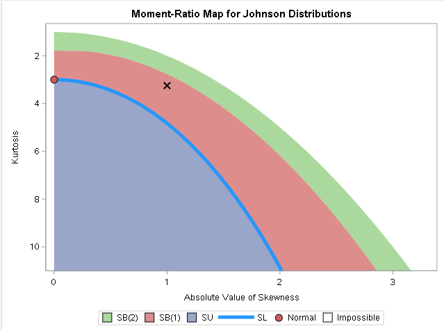
PROC SIMSYSTEM produces several output tables and graphs. My favorite is the moment-ratio diagram, which shows the (skewness, kurtosis) values that are covered by the members of the Johnson family. The diagram (shown to the right) shows:

• The red dot at (0, 3) represents the normal distribution.
• The pale blue-gray area is the (skewness,kurtosis) region that is covered by the unbounded Johnson SU distributions.
• The bright blue curve is the (skewness,kurtosis) curve that is covered by the lognormal distributions (SL).
• The reddish-brown region is covered by the unimodal Johnson SB distributions (SB(1)).
• The bright green region is covered by the bimodal Johnson SB distributions (SB(2)).
• The X markers indicate the Johnson SB distributions that correspond to the specified moments. The moments in this example correspond to a unimodal SB distribution.

The ParameterEstimates table shows the estimated parameters for the fitted Johnson SB distribution, as shown below:

The table shows that Johnson SB distribution has four parameters. The distribution that has the specified moments has the parameters Delta=0.742, Gamma=1.028, Shift=-0.027, and Scale=1.006. (In PROC UNIVARIATE, the threshold parameter, Shift, is called Theta, and the Scale parameter is called Sigma.) This is the fitted model. To create new simulated sample, use these values for the SB distribution.

The output also includes a PDF of a centered-and-scaled version of the Johnson SB distribution (not shown). The next section shows how to use the ParameterEstimates data set to construct the non-centered and non-scaled PDF. The non-centered version is a better way to compare the distribution to the original histogram of the data.

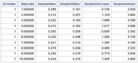
I suppressed the display of the Moments table, which shows the sample moments for the 10,000 simulated data set from the Johnson SB distribution. Instead, I wrote the sample moments to a data set. You can use PROC PRINT to look at the descriptive statistics for a few of the samples:

proc print data=Moments(obs=10) noobs; 
   var SimIndex Replicate SampleMean SampleStdDev SampleSkewness SampleKurtosis;
run;

The output shows that the sampling variability of the mean and standard deviation statistics is relatively small whereas the variability is much greater for the skewness and kurtosis statistics. This is typical behavior because the standard error of the mean is smaller than for higher-order moments. You can use the sample moments to visualize the sampling distribution of the skewness and kurtosis statistics.

Lastly, the procedure simulates 10,000 random samples of size N=50 from the SB distribution and puts them into a CAS table for use in a simulation study. Ransdell and Tobias (2020, pp. 13-16) show an example of using the simulated samples in a financial application.

Visualize the Johnson SB Distribution

As shown in a previous article, you can use the DATA step and PROC SGPLOT to visualize the PDF for the Johnson SB distribution, as follows:

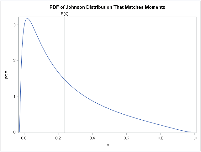
data JohnsonPDF;
set JohnsonParams(keep= Delta Gamma Shift Scale);
sqrt2pi = sqrt(2*constant('pi'));
theta = shift; sigma = scale;
c = delta / (sigma * sqrt2pi);
do x = theta+1E-6 to theta+sigma by 0.005;
   w = (x-theta) / sigma;
   t = (x - theta) / (theta + sigma - x);
   PDF = c / (w*(1-w)) * exp( -0.5*(gamma + delta*log(t))**2 );
   output;
end;
keep x PDF;
run;
 
title "PDF of Johnson Distribution That Matches Moments";
proc sgplot data=JohnsonPDF;
   series x=x y=PDF;
   refline 0.235 / axis=x label="E[X]";
run;

A few features are noteworthy. First, the support of the distribution is not [0,1]. Rather, the domain is [Shift, Scale+Shift], where Shift and Scale are the parameter estimates for the Johnson SB distribution. For this example, the support of the distribution is [-0.0275, 0.9783]. This is in contrast to a model that uses the Beta distribution, for which the support is always (0,1). Consequently, the SB model might not be appropriate is the real data must always be in the interval [0,1].

Notice also that the mode is in the interior of the interval of support. If you were to fit the data to a Beta distribution, the resulting model is Beta(0.705, 2.295) which has an infinite density at x=0. If you have domain knowledge about the true distribution of the data, that might help you decide whether the SB or the Beta model is more faithful to the true data-generating process.

Summary

PROC SIMSYSTEM is a SAS Viya procedure that can fit distributions in the Pearson and Johnson systems. It is easy to use because it requires only that you specify the moments of the distribution. Each unique (skewness, kurtosis) value corresponds to a unique distribution in the system. The example in this article demonstrates an example that uses the Johnson system. You can use the procedure to select a distribution that has the same moments and to simulate random samples from that distribution. Although not shown in this article, you can specify a grid of (skewness, kurtosis) values, which enable you to conduct simulation studies that use a wide variety of distributional shapes and characteristics.

For more information about the SIMSYSTEM procedure and moment-ratio diagrams, see the following references:

• Ransdell, B. and Tobias, R. (2020) "Introducing PROC SIMSYSTEM for Systematic Nonnormal Simulation".
• "The SIMSYSTEM Procedure" SAS Visual Statistics: Procedures
• Wicklin, R. (2013) Simulating Data with SAS, Chapter 20, "Moment Matching and the Moment-Ratio Diagram."
• Wicklin, R. (2020) "The moment-ratio diagram", The DO Loop blog.