A convolution is a mathematical operation on two discrete sequences (or continuous functions) that produces a new sequence (or function). In probability and statistics, a convolution is closely associated with the concept of a "moving window," which time series analysts often call a "filter." If you have ever smoothed a time series, created a kernel density estimate, or calculated the distribution of the sum of two independent random variables, you have used a convolution, whether you realized it or not.
This article provides the mathematical background for a discrete convolution operation. It discusses a SAS IML function, DFCONV, that you can use to compute a discrete convolution. The convolution operation is illustrated by using two classical statistical applications. The first is the sum of two independent discrete random variables. The second is the computation of a moving average for a time series.
The formula for a discrete convolution
The convolution operation comes in two forms: a continuous convolution that operates on functions, and a discrete convolution that operates on sequences. This article discusses only the discrete convolution operator. The discrete convolution operator is a binary operation on two sequences, u and v. It produces a new sequence, denoted u*v, by using multiplication and addition of the terms in the original sequences. Each element of u*v is a dot product for a subsequence of elements in u and v.
In math, the two sequences are usually indexed starting at 0. That is, u = {u0, u1, ..., uM-1} and v = {v0, v1, ..., vN-1}. The sequence u has M elements; the sequence v has N elements. The full convolution u*v is a new sequence that has M+N-1 elements (indexed from 0 to M+N-2). The k-th element of u*v, denoted as (u*v)(k), is defined as:
\( (u*v)(k) = \sum_{j=\max(0, k-N+1)}^{\min(k, M-1)} u(j)v(k-j) \)
If you adopt the convention that the sequences are infinite and that the unspecified terms of the sequences are zero,
this formula can be written more simply:
\( (u*v)(k) = \sum_{j=-\infty}^{\infty} u(j)v(k-j) \)
This version makes it look more like the continuous convolution operator, which replaces the summation with an integral.
The convolution is commutative, so you can also use u(k-j)v(j) in the formula. I use this fact in the section about time-series smoothing.
Computing a convolution: The DFCONV function in SAS IML
In Appendix A, I show how to "manually" compute a discrete convolution between two vectors in the SAS IML language. (The SAS IML language uses one-based indexing, so the indices in the implementation are slightly different than in the formula that I showed in the previous section.) But, you don't need to write any code to use a convolution. The SAS IML language provides a built-in function, the DFCONV function, which automatically computes the convolution and a few useful variations. The documentation shows the formula for vectors that use one-based indexing. The 'DF' prefix stands for 'Digital Filter', which is the name that electrical engineers use for operations that process digital signals.
Let's look at a simple numeric example. Suppose that u = {1,2,3} and v = {4,5,6,7,8} are vectors of length M=3 and N=5, respectively. You can use the DFCONV function to compute the convolution y = u*v, as follows:
proc iml; u = {1,2,3}; v = {4,5,6,7,8}; y = dfconv(u,v); print y; |

Appendix A provides the step-by-step manual computations that verify that the output is correct. Notice that the output length is N + M - 1 = 3 + 5 - 1 = 7.
Example 1: The sum of two independent random variables
An example of a discrete convolution in probability theory is the distribution of the sum of two independent rolls of dice. When you sum two independent random variables, the distribution of the sum is the convolution of their individual probability distributions.
A classic example is two fair six-sided dice. Let X and Y be the outcomes of the two dice. Both follow a discrete uniform distribution. The probability mass function (PMF) for a single die can be represented as a vector of probabilities for the outcomes 1 through 6. Thus, u = {1/6, 1/6, 1/6, 1/6, 1/6, 1/6} and v = {1/6, 1/6, 1/6, 1/6, 1/6, 1/6} are the PMFs.
Let Z = X + Y be the sum of the dice faces. The random variable Z takes on values in the range 2, 3, 4, ..., 12. The probability that Z=2 is relatively small because there is only one way ("snake eyes") for that sum to occur. In contrast, there are six equally likely ways for the sum to be 7: 1+6, 2+5, 3+4, 4+3, 5+2, and 6+1. In general, if the sum of the two dice is s, and if X=k, then we know that second die has the value s-k. Thus, to find the probability that Z=s, we must sum the probabilities that X=k and Y=s-k for k=1..6.
Because X and Y are independent, the probability that X=k and Y=s-k is the product
P(X=k)*P(Y=s-k). To find the complete probability that Z=s, we sum over all the ways that
the sum s can occur. This leads to the formula
\( P(Z = s) = \sum_{k} P(X = k) P(Y = s - k) \)
The right side of the formula is the k_th element of a convolution.
Thus, to find the probability distribution of the sum of two dice, you can convolve
the PMFs for each die.
You can use the DFCONV function in IML to find the distribution of the sum of two six-sided dice, as follows:
/* Example: Discrete convoution of rolling two fair six-sided dice */ proc iml; prob_d6 = {1,1,1,1,1,1} / 6; /* PMF of six-side fair die */ prob_2dice = dfconv(prob_d6, prob_d6); /* PMF of sum of two dice */ print prob_2dice[r=(2:12) F=FRACT12.]; |
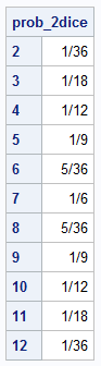
The PMF for each die has six elements. Thus, the convolution is a vector of length 6 + 6 - 1 = 11, which corresponds to the sums 2-12. The PMF of the sum is the familiar triangular distribution, which peak at the sum of 7 with a probability of 6/36 or 1/6.
If you want the sum of three dice, you can convolve the distribution of the sum with the distribution of another fair die, as follows:
/* Want three dice? Convolve the probability distribution for a six-sided die with the distribution for two independent dice. */ prob_3dice = dfconv(prob_d6, prob_2dice); print prob_3dice[r=(3:18) F=FRACT12.]; |

You can continue this process as many times as you like. You can compare the result to the classical formula for rolling n six-sided dice. If the dice are not fair, you can replace the vectors u and v with other vectors that specify the probability for each face.
Example 2: Moving averages in time series
A second application of convolution is smoothing a sequence of data points by using a moving window analysis. When you apply a moving average, you convolve a short sequence (the filter or kernel) with a longer data sequence. I have previously discussed how to compute a moving average and how to compute a moving average in SAS by using PROC EXPAND or SAS IML functions.
In the previous post, I use PROC EXPAND to find two different (backward) moving averages of the monthly price of IBM stock in the late 1990s and early 2000s. The following SAS statements smooth 120 prices and create a graph that overlays the scatter plot, a moving average, and a weighted moving average. See the previous article for an explanation and discussion.
/* Example from https://blogs.sas.com/content/iml/2016/01/27/moving-average-in-sas.html */ title "Monthly IBM Stock Price"; proc sort data=sashelp.stocks(where=(STOCK='IBM') rename=(Date=t Close=y)) out=Series(keep=t y); where ('01JAN1996'd <= t <= '31DEC2005'd); by t; run; /* create three moving average curves. Use the TRIM option to remove edge effects and compute only the "middle" of the smoother. */ proc expand data=Series out=out method=none; id t; convert y = MA / transout=(movave 5 trim 5); /* backward MA(5) */ convert y = WMA / transout=(movave(1 2 3 4 5) trim 5); /* backward WMA */ run; proc sgplot data=out cycleattrs; scatter x=t y=y; series x=t y=MA / name='MA' legendlabel="MA(5)"; series x=t y=WMA / name='WMA' legendlabel="WMA(1,2,3,4,5)"; keylegend 'MA' 'WMA'; xaxis display=(nolabel) grid; yaxis label="Closing Price" grid; run; |
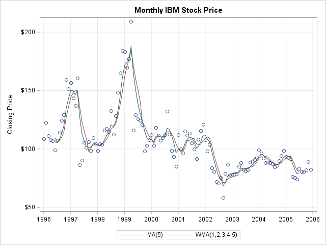
PROC EXPAND has various options to deal with averages at the beginning and end of the sequence, where there are not enough points to perform a full convolution. By default, it adjusts the width of the moving window. To avoid a discussion of edge effects, I used the TRIM option to output missing values for the first and last five averaged values. Thus, the graph shows smoothers that do not predict values for the first five and the last five observations. I will do the same after convolving the window and the data. In this way, I avoid a distracting discussion about why the default behavior of PROC EXPAND deviates from the mathematical definition of a convolution.
Let's perform the moving average computation in SAS IML by using a convolution. We want the filter elements to sum to unity, A simple backward moving average with a window width of 5 corresponds to a filter with values u={1,1,1,1,1}/5. The backward weighted moving average corresponds to u={5,4,3,2,1}/15. Notice that the order of the elements in the weighted kernel are reversed from the PROC EXPAND order. Why? Well, the mathematical definition of a convolution flips the kernel shape (that is, it uses u(k-j) to compute the k_th smoothed point). We therefore need to manually reverse the elements in u before calling the DFCONV function so that the output agrees with the backward moving average from PROC EXPAND.
/* perform a similar computation by using convolution */ proc iml; /* read the data into v */ use Series; read all var "y" into v; close; u = {1,1,1,1,1} / 5; /* MA(5) */ MA = dfconv(u, v); /* reverse the filter elements to match the PROC EXPAND output for a backward MA */ u = {5,4,3,2,1} / 15; /* WMA(1,2,3,4,5) */ WMA = dfconv(u, v); /* We want to compare with PROC EXPAND. The PROC 1) outputs N elements. 2) has special handling for the first and last N obs. */ M = nrow(u); N = nrow(v); MA = MA[1:N]; /* keep only N elements */ WMA = WMA[1:N]; firstObs = 1:M; lastObs = (N-M+1):N; MA [firstObs||lastObs] = .; /* set the first/last obs to missing */ WMA[firstObs||lastObs] = .; create IML_MA var {'MA' 'WMA'}; append; close; QUIT; proc compare base=out(keep=MA WMA) compare=IML_MA method=absolute criterion=1E-12; run; |
                                       Observation Summary

                                  Observation      Base  Compare

                                  First Obs           1        1
                                  Last  Obs         120      120

                 Number of Observations in Common: 120.
                 Total Number of Observations Read from WORK.OUT: 120.
                 Total Number of Observations Read from WORK.IML_MA: 120.

                 Number of Observations with Some Compared Variables Unequal: 0.
Number of Observations with All Compared Variables Equal: 120. |
The IML values (computed by using a convolution) agree with the PROC EXPAND values to within 1E-12. (In fact, the largest difference for this example is 5.68E-14.) If we had not used the TRIM option in PROC EXPAND, then there would be differences in the first few observations because PROC EXPAND uses a varying-width kernel near the beginning and end of the data series.
Summary
This article discusses the mathematical definition of a discrete convolution operator. In SAS, you can use the DFCONV function in SAS IML to convolve two vectors of arbitrary lengths. The result is a new longer vector. The convolution operator is illustrated by using two examples: the distribution of the sum of two six-sided dice, and the smoothing of a time series by using a moving average.
Appendix A: Manual computation of a discrete convolution
This appendix shows a simple manual computation of discrete convolution for two vectors. It is presented so that you can compare the output of the DFCONV function with a function that directly implements the convolution formula.
Suppose you define a vector, u={1,2,3}, which has M=3 elements, and a vector, v={4,5,6,7,8}, which has N=5 elements. If you want to compute their convolution, y=u*v, you can use the following manual computations. These computations assume zero-based indexing. For this problem, the convolution has M+N-1 = 7 elements:
y[0] = u[0]v[0] = 1*4 = 4 y[1] = u[0]v[1] + u[1]v[0] = (1*5) + (2*4) = 13 y[2] = u[0]v[2] + u[1]v[1] + u[2]v[0] = (1*6) + (2*5) + (3*4) = 28 y[3] = u[0]v[3] + u[1]v[2] + u[2]v[1] = (1*7) + (2*6) + (3*5) = 34 y[4] = u[0]v[4] + u[1]v[3] + u[2]v[2] = (1*8) + (2*7) + (3*6) = 40 y[5] = u[1]v[4] + u[2]v[3] = (2*8) + (3*7) = 37 y[6] = u[2]v[4] = 3*8 = 24 |
Thus, the convolution y=u*v is a new vector, y = {4,13,28,34,40,37,24}.
There are two issues when turning this into a computation. First, the IML language uses one-based indexing, not zero-based. Second, a naive implementation would use a pair of nested loops and perform scalar multiplication and addition, which is inefficient in a vectorized language. A better implementation is to use a dot product to perform the sums of the products of subsequences. After the first few elements of the vector v, the dot products will always use subsequences of length M, which is the length of u.
The following computation implements the definition of the discrete convolution formula.
proc iml; /* y = conv(u,v) convolves column vectors u and v. Algebraically, convolution is the same operation as multiplying the polynomials whose coefficients are the elements of u and v. */ start conv_manual(u,v); m = nrow(u); n = nrow(v); ny = m + n - 1; y = j(ny, 1, 0); do k = 1 to ny; idx = max(1, k+1-n):min(k,m); y[k] = u[idx]` * v[k + 1 - idx]; end; return (y); finish; /* test the computation */ u = {1,2,3}; v = {4,5,6,7,8}; y1 = conv_manual(u,v); /* compare to the built-in IML function */ y2 = dfconv(u,v); print y1 y2; |
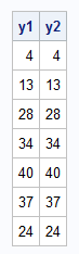
Notice the statement, idx = max(1, k+1-n):min(k,m), which selects the indices to use for the dot product. This statement corresponds to the summation limits in the mathematical formula earlier. In the formula, the lower limit of summation is max(0, k-N+1) and the upper limit is min(k, M-1). The IML statement adjusts these limits to account for 1-based indexing.
Appendix B: Convolution as matrix-vector multiplication
Incidentally, the first time I saw a convolution operator was in a course in Linear Algebra where it was presented as an example of a bilinear operator between two vector spaces. Accordingly, you can represent a convolution as a matrix-vector multiplication where the matrix T=T(v) is a Toeplitz-type matrix of the appropriate dimension and padded with zeros. In honor of my now-deceased Cornell math professor, Keith Dennis, I'll show how to construct the matrix and use it to compute a convolution in IML:
ny = nrow(v) + nrow(u) - 1; Tv = j(ny, nrow(u), 0); do i = 1 to nrow(u); Tv[i:(i+nrow(v)-1),i] = v; /* create a Toeplitz-type matrix by copying v into columns */ end; y3 = Tv*u; /* matrix-vector multiplication */ print Tv, y3; |

In practice, there is no advantage to construct a large matrix and perform matrix-vector multiplication. You can save RAM memory and compute a series of dot products instead. Nevertheless, it's a cool result!