The classical multivariate normal (MVN) distribution is a standard model for correlated data. It is a simple model, it is easy to fit the MVN model to data, and the parameters in the model (locations and correlations) are intuitive. Of course, normality is a strong assumption that is not always satisfied by real-world data, which might have skewness and extreme-tail behavior. The normal distribution (whether univariate or multivariate) is an example of a "thin-tailed" model because the probability of an extreme value declines to zero exponentially fast as a function of the distance to the center of the data.
Certain fields, such as quantitative finance and climatology, routinely use models with thicker tails. If you need to analyze data that have "heavy tails," one possible choice is the multivariate t (MVT) distribution. The MVT distribution has a parameter, ν, that controls the tail thickness. For historical reasons, ν is called the degrees-of-freedom parameter. When used for inferential statistics, the parameter is an integer. However, for the MVT distribution, ν is a shape parameter that is not restricted to integer values. For small values of ν, the MVT provides a heavy-tailed alternative to the MVN distribution. As ν → ∞, the MVT distribution approaches the multivariate normal distribution.
I have previously written about how to visualize the multivariate t distribution in SAS, including how to evaluate the multivariate t PDF and how to generate random variates from MVT by using the RANDMVT function in SAS IML software. This article discusses how to compute the cumulative distribution function (CDF) for the multivariate t distribution. The CDF requires computing a high-dimensional integral. The article includes a SAS IML function that evaluates the CDF for the multivariate t distribution in two dimensions.
A general formula for the CDF of the multivariate t distribution
This section presents the advanced math that enables you to compute the CDF for the multivariate t (MVT) distribution. If you prefer programming over math, you can skip to the next sections.
The book Computation of Multivariate Normal and t Probabilities (Genz and Bretz, 2009) shows that you can obtain the CDF of the standard MVT(Σ, ν) distribution as an integral of the CDF of the MVN(0, Σ) distribution. The goal is to evaluate the probability that a k-dimensional random variable X ~ MVT(Σ, ν) is in a hyper-rectangular region: P(a1 < X1 < b1, a2 < X2 < b2, ..., ak < Xk < bk). Here Σ is a k x k positive semidefinite covariance matrix that defines the correlations between the components of X.
The vectors a = (a1, a2, ..., ak) and b = (b1, b2, ..., bk) define the rectangular region. To obtain the probability that a random variate is in this region, you use the components of a for the lower limits of integration, and the components of b for the upper limits. The components of a can be -∞, and the components of b can be +∞.
Although you can define the probability directly as a multivariate integral over the hyper-rectangular region, Genz and Bretz show that you
can also compute the probability by integrating a function that includes the CDF for a MVN distribution.
The first formula appears on p. 3 and is listed as Eqn 1.3.
The formula shows how to compute the MVT CDF by integrating a related CDF for the MVN distribution over the
infinite interval (0, ∞). Then,
in Chapter 4 (Eqn 4.6, p. 32-33),
Genz and Bretz show that you can transform the integral on the infinite interval (0, ∞) into an equivalent integral on (0,1).
The formula is:
\(
T_k(\mathbf{a}, \mathbf{b}; \boldsymbol{\Sigma}, \nu) =
\int_{0}^{1} \Phi_k \left( \frac{\chi_\nu^{-1}(t)\mathbf{a}}{\sqrt{\nu}}, \frac{\chi_\nu^{-1}(t)\mathbf{b}}{\sqrt{\nu}};
\boldsymbol{\Sigma} \right) dt
\)
In this formula:
- Tk(a, b; Σ, ν) is the CDF function for the MVT distribution. It gives the probability that a random variate from MVT(Σ, ν) is in the region defined by the vectors a and b.
- Φk is the MVN CDF in dimension k. \(\Phi_k (\mathbf{L}, \mathbf{U}; \boldsymbol{\Sigma})\) is the probability that a random variable from the centered MVN distribution is in the hyper-rectangular region defined by the lower-limit vector, L, and the upper-limit vector, U. The vector L = \(\frac{\chi_\nu^{-1}(t)\mathbf{a}}{\sqrt{\nu}}\), and U = \(\frac{\chi_\nu^{-1}(t)\mathbf{b}}{\sqrt{\nu}}\), where t is the dummy integration variable in (0,1).
- χν-1 is the quantile function for the chi distribution. If you've never heard of the chi distribution, don't worry. It is closely related to the familiar chi-square distribution. In fact, if Y ~ χ2(ν) is distributed as a chi-squared distribution with ν degrees of freedom, then X = sqrt(Y) is distributed as a chi distribution with ν degrees of freedom. This definition means that you can use the QUANTILE("CHISQ") distribution in Base SAS to compute the quantile function of the chi distribution. You simply take the square-root of the resulting quantile!
This formula enables you to compute the exact CDF of a MVT distribution by integrating a function that involves only the (transformed) probability of the MVN distribution over the interval (0,1). In SAS, you can use the PROBBNRM function to evaluate 2-D MVN CDF. And SAS IML software enables you to integrate arbitrary functions! So, let's write a SAS IML function that uses the formula to evaluate probabilities for the 2-D MVT distribution. The function will enable you to compute exact CDF values in this case.
The CDF of the bivariate t distribution in SAS
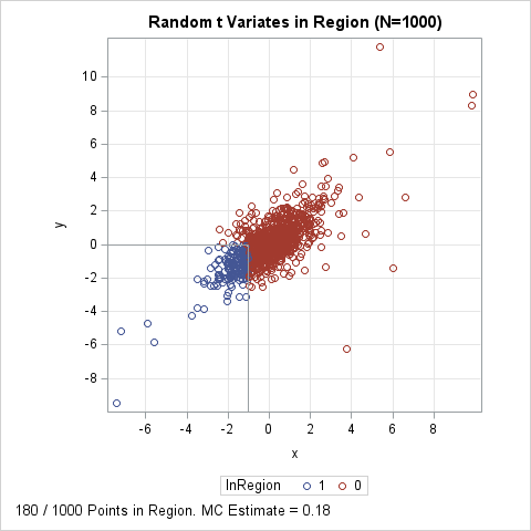
The formula for Eqn 4.6 provides the CDF on any rectangular region. However, for ease of presentation, I will present the simpler case of the "left-tailed" CDF in 2-D, which is the probability that a random variable is in the region (-∞, b1)x(-∞, b2). In other words, I will set the vector of lower limits to a = (-∞, -∞). This computation can be used to compute the probability of general rectangular regions.
A left-tailed region is shown in the image to the right. In the image, I generated 1,000 random variates according to a bivariate t distribution with ν=5 degrees of freedom. Of those points, 180 of them fall into the region {(x,y) | x < -1, y < 0}, which means that a Monte Carlo estimate for the probability is 0.18. Let's use the formulas in the previous section to obtain a better estimate of the probability.
You can use the QUAD routine in the SAS IML language to perform numerical integration. It is helpful to use the PEAK= option to tell the QUAD routine to avoid evaluating the integral near the boundary of the integration region. The following IML program defines and store three functions. The BVT_CDF is the top-level function that evaluates the bivariate t CDF. 'BVT_CDF' is short for 'bivariate t CDF'.
/* A useful result in computational statistics is Eqn 1.3 and Eqn 4.6 in Genz and Bretz (2009, Computation of Multivariate Normal and t Probabilities, p. 3, 32-33). The equation shows that you can compute any multivariate t CDF by computing an integral that uses the multivariate normal (MVN) CDF. Specifically, Eqn 4.6 shows that you can use the quantile of the CHI distribution (CHI, not chi-squared!) to transform Eqn 1.3 into an integral on the interval (0,1). */ proc iml; /* truncate every element of x into the interval [ab[1], ab[2]]. See https://blogs.sas.com/content/iml/2026/02/04/clip-values.html */ start TruncateToRange(x, ab); a = ab[1]; b = ab[2]; return( (a <> x) >< b ); finish; /* Define the integrand from Equation (4.6) in Genz (2009) by calling the PROBBNRM function in Base SAS to compute the bivariate normal CDF. For numerical reasons, limit the evaluation of PROBBNRM to [-10,10] in each coordinate. In case nu is large, use the exp(log(.)) trick to evaluate the constants. */ start BVT_CDF_Integrand(t) global(g_b, g_rho, g_nu); b = g_b; rho = g_rho; nu = g_nu; if t<=0 then s=0; else if t>=1 then s=1E6; else s = sqrt( quantile("ChiSq", t, nu)); w = s * b / sqrt(nu); w = TruncateToRange(w, {-10, 10}); /* protect against floating point underflow; max value is 10 */ f = probbnrm(w[1], w[2], rho); return( f ); finish; /* wrapper function to set global variables and call the integration */ start BVT_CDF(b, rho, nu) global(g_b, g_rho, g_nu); g_b = b; g_rho = rho; g_nu = nu; call quad(BVT_prob, "BVT_CDF_Integrand", {0 1}) peak=0.1; return( BVT_prob ); finish; store module=(TruncateToRange BVT_CDF_Integrand BVT_CDF); QUIT; |
Having defined the functions, you can now call them to compute the CDF for the bivariate t distribution, as follows:
proc iml; load module=_all_; /* call the BVT_CDF with different values of b and nu */ b = {-1, 0}; /* upper limits for X1 and X2 */ rho = sqrt(2)/2; /* correlation */ nu = 5; /* DOF */ /* first, compute the probability for the MVN distribution */ BVN_prob = probbnrm(b[1], b[2], rho); print (b`)[c={'b1' 'b2'}] rho BVN_prob[L="Bivariate Normal CDF"]; /* compare to the MVT probability (nu=5) */ BVT_prob = BVT_CDF(b, rho, nu); print nu (b`)[c={'b1' 'b2'}] rho BVT_prob[L="Bivariate t CDF"]; |
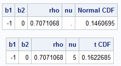
For these calculations, we assume that two random variables have the correlation 0.7071. The first output uses the built-in PROBBNRM function in SAS to compute the probability P(Z1 < -1, Z2 < 0) for Z ~ MVN(0, R), where R is the correlation matrix with off-diagonal elements ρ. The output shows the bivariate normal CDF at (-1,0) is 0.146. In contrast, the CDF for the bivariate t distribution with 5 DoF is 0.162 because a t distribution has heavier tails. This is the probability P(T1 < -1, T2 < 0) for T ~ MVT(0; R, ν). This value is much more accurate than the Monte Carlo estimate shown in the previous section. In addition, the Monte Carlo estimate suffers from variability: If you choose a different set of 1,000 random points, you will get a different Monte Carlo estimate. In contrast, the integration method is deterministic and highly accurate.
If you reverse the correlation of the variables, you get two negatively correlated variables. You can compute the CDF probability for the MVT distribution with ρ = -0.7071 by using the following call:
rho = -sqrt(2)/2; /* correlation */ BVT_prob2 = BVT_CDF(b, rho, nu); print nu (b`)[c={'b1' 'b2'}] rho BVT_prob2[label="Bivariate t CDF"]; |
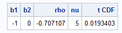
The probability in the region is about 0.019, which is smaller than for the positively correlated variables. You can understand this smaller number by looking back at the scatter plot in the previous section. That scatter plot has a southwest-to-northeast orientation. When you reverse the correlation, the analogous scatter plot will have a southeast-to-northwest orientation. (Mentally flip the scatter plot about the vertical line x=0.) The new scatter plot will have only a small proportion of points (about 19 per thousand) that fall into the specified region.
Summary
This article shows a direct method to evaluate the CDF for the bivariate t distribution in SAS. The computation relies on a mathematical result in Genz and Bretz (2009), which shows that you can evaluate the probability that a MVT variable (in any dimension) is in a rectangular region by integrating the CDF for the MVN distribution over the interval (0, 1). To simplify the presentation, I showed the special case of computing the CDF for the bivariate t distribution on left-tailed regions {(T1,T2) | T1 < b1, T2 < b2}, where T = (T1,T2) is a random variable distributed as MVT(Σ, ν). You can use this left-tail probability to compute the probability in any other 2-D rectangular region.
It is difficult to compute the exact CDF of the MVN distribution in k dimensions when k > 2. However, you can use the formula and numerical methods such as quasi-Monte Carlo computations to compute the CDF of the MVT distribution to high precision.