A previous article shows how to compute the probability density function (PDF) for the multivariate normal distribution. In a similar way, you can compute the density function for the multivariate t distribution. This article discusses the density function for the multivariate t distribution, shows how to compute it, and visualizes the density for a bivariate distribution in two different ways.

As for all multivariate computations, the computations are simpler when you express the formulas in terms of matrices and vectors. This article uses the SAS/IML language to evaluate the multivariate t distribution.

A comparison of the normal and t distributions

Before discussing multivariate distributions, let's recall the univariate t distribution and compare its shape to the standard normal distribution. The density of the univariate t distribution with $\nu$ degrees of freedom has the following formula:
$f(x)=\frac { \Gamma((\nu +1)/2) } { \Gamma(\nu/2) \sqrt{\nu \pi} } \left(1+{\frac {x^{2}}{\nu }}\right)^{-(\nu +1)/2}$
Here, $\Gamma(\cdot)$ is the gamma function.

The t distribution is symmetric and converges to the standard normal distribution as $\nu \to \infty$. For any finite value of $\nu$, the t density function has more weight in the tails and, consequently, less weight near the center of the distribution. The following SAS DATA step uses the PDF function to compute the density function for the standard normal distribution and the t distribution with $\nu=10$ degrees of freedom. The call to PROC SGPLOT overlays the two density curves:

/* compare the univariate normal and t density curves (DF=10) */
data Compare;
DF = 10;
mu = 0; sigma = 1;
do x = -4 to 4 by 0.1;
   Normal = pdf("Normal", x, mu, sigma);
   T = pdf("t", x, DF);
   output;
end;
run;
 
title "Comparison of Normal and t Distributions";
proc sgplot data=Compare;
  series x=x y=Normal;
  series x=x y=T / lineattrs=(thickness=2);
run;

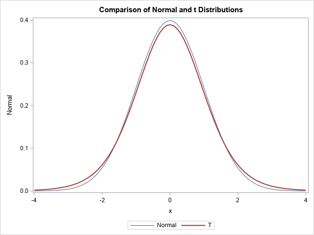
As expected, the density curve for the t distribution is lower at the origin and higher in the tails, as compared with the standard normal distribution. This relationship is also true for the multivariate distributions: the multivariate t distribution looks a lot like the multivariate normal distribution but has less density near the center of the distribution and more density in the tails. In terms of a random sample, this means that data drawn from a multivariate t distribution has a wider spread: fewer points are near the center and more points are away from the center, as shown in the next section.

Empirical density of the bivariate t distribution

The SAS/IML language supports random sampling from the multivariate normal and t distributions. You can use the RANDNORMAL function to sample from a multivariate normal distribution. In dimension p, the parameters are μ and Σ. The μ parameter is a mean vector of length p. The Σ parameter is a p x p covariance matrix. The multivariate t distribution also uses those parameters, as well as a scalar parameter that represents the degrees-of-freedom. The following SAS/IML program simulates 1,000 random observations from the bivariate normal and bivariate t (DF=10) distributions. The observations are written to a SAS data set, and PROC KDE is used to visualize the density of the bivariate scatter plot:

proc iml;
call randseed(123);
N = 1000;
mu = {1 2};
Sigma = {2 1, /* correlation coefficient is sqrt(2) */
         1 1};
DF = 10;
Z = randnormal(N, mu, Sigma);   /* N obs from the MVN(mu, Sigma) distrib */
T = randmvt(N, DF, mu, Sigma);  /* N obs from the MV t(DF) distrib */
 
A = Z || T;
create Sample from A[c={z1 z2 t1 t2}];
   append from A;
close;
QUIT;
 
/* Use PROC KDE to visualize bivariate density. See
   https://blogs.sas.com/content/iml/2019/09/18/visualize-density-bivariate-data.html */
%macro MakeDensityPlot(var1, var2);
   data Have; set Sample(keep=&var1 &var2); run;
   proc kde data=Have;
     bivar  &var1 &var2 / bwm=1 ngrid=250 plots=none noprint;
     score data=Have out=Out(rename=(value1=&var1 value2=&var2));
   run;
   proc sort data=Out;  by density;  run;
   proc sgplot data=Out;
      styleattrs wallcolor=verylightgray;
      scatter x=&var1 y=&var2 / colorresponse=density colormodel=ThreeColorRamp
                         markerattrs=(symbol=CircleFilled) transparency=0.5;
      xaxis grid values=(-5 to 7); 
      yaxis grid values=(-3 to 7);
   run;
%mend;
 
title "Density of Multivariate Normal Sample";
%MakeDensityPlot(z1, z2)
title "Density of Multivariate t Sample (DF=10)";
%MakeDensityPlot(t1, t2)

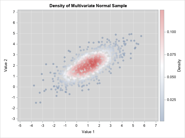
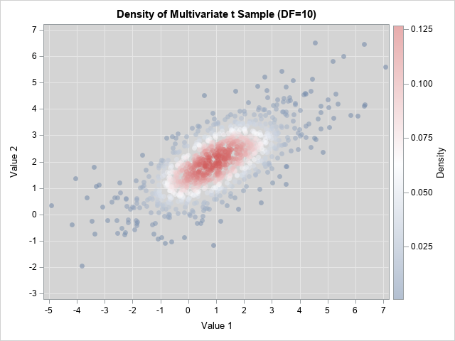
The graphs are both scatter plots, but the observations have been colored according to an estimate of the bivariate density. You can see that the points for the bivariate normal distribution are more concentrated near the origin (the center of these data) and have less variation compared to the points for the bivariate t distribution. In both cases, the Σ parameter provides a way to model the correlation between the variables.

These graphs show the empirical density for a random sample. For very large samples, the empirical density should be close to the probability density, which is presented in the next section.

Probability density for the multivariate t distribution

The standard formula for the univariate t distribution does not have a location or scale parameter, but you can add those parameters so that the t distribution is analogous to the univariate normal distribution. In the earlier DATA step, you could modify the PDF by using the expression
T = 1/sigma * pdf("t", (x-mu)/sigma, DF);

In a similar way, you can add location and covariance parameters to the multivariate t distribution. Recall that the multivariate normal PDF contains the expression d²=(x-μ)^TΣ^-1(x-μ), where d is the Mahalanobis distance between the multidimensional vector x and the mean vector μ. The same expression appears in the following formula for the density of the multivariate t distribution:
$f(x)=\frac {\Gamma ((\nu +p)/2) } {\Gamma (\nu/2) (\nu \pi)^{p/2} |\Sigma|^{1/2} } \left(1+ \frac{1}{\nu} (x - \mu)^T \Sigma^{-1} (x - \mu)\right)^{-(\nu +p)/2}$

The SAS/IML language supports the MAHALANOBIS function, which enables you to compute that quadratic term quickly and efficiently. The following SAS/IML module defines the PDF for the multivariate t distribution. For comparison, I also define the PDF for the multivariate normal distribution. I then evaluate the PDFs on a uniform bivariate grid of values and write the values to a data set. For later use, the program also evaluates the logarithm of the densities.

/* evaluate multivariate t density */
proc iml;
/* Probability density for the MV normal distribution. See
   https://blogs.sas.com/content/iml/2012/07/05/compute-multivariate-normal-denstity.html */
start MVNormalPDF(x, mu, cov);
   p = nrow(cov);
   const = (2*constant("PI"))##(p/2) * sqrt(det(cov));
   d = Mahalanobis(x, mu, cov);
   phi = exp( -0.5*d##2 ) / const;
   return( phi );
finish;
 
/* Probability density for the multivariate t distribution */
start MVTPDF(x, nu, mu, cov );   /* DF = nu degrees of freedom */
   p = nrow(cov);
   pi = constant("PI");
   np2 = (nu+p)/2;
   const = Gamma(np2) / (Gamma(nu/2) * (nu*pi)##(p/2) * sqrt(det(cov)));
   d = Mahalanobis(x, mu, cov);
   f = const * (1 + d##2/nu)##(-np2);
   return( f );
finish;
 
/* 2-D example */
mu = {1 2};
Sigma = {2 1, /* correlation coefficient is sqrt(2) */
         1 1};
 
xx = do(-5, 7, 0.2);
yy = do(-3, 7, 0.2);
xy = ExpandGrid(xx, yy);
 
NormalDensity = MVNormalPDF(xy, mu, Sigma);
DF = 10;
TDensity = MVTPDF(xy, DF, mu, Sigma);
 
logNormal = log10(NormalDensity); /* Optional: Compute LOG10 of densities */
logT = log(TDensity);
x1 = xy[,1]; x2 = xy[,2];
create BivarDensity var {"x1" "x2" "NormalDensity" "TDensity" "logNormal" "logT"};
   append;
close;
QUIT;

You can use a contour plot to visualize the bivariate normal a bivariate t densities:

/* Define and use the ContourPlotParm GTL template from 
   https://blogs.sas.com/content/iml/2012/07/02/create-a-contour-plot-in-sas.html */
proc sgrender data=BivarDensity template=ContourPlotParm;
dynamic _TITLE="Bivariate Normal Density, corr=sqrt(2)"
        _X="x1" _Y="x2" _Z="NormalDensity";
run;
 
proc sgrender data=BivarDensity template=ContourPlotParm;
dynamic _TITLE="Bivariate t Density, corr=sqrt(2), DF=10"
        _X="x1" _Y="x2" _Z="TDensity";
run;

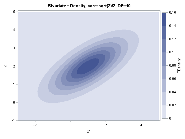
I don't know about you, but I cannot see a difference between the contour plots on this scale. Recall that for the 1-D distributions, the density curves were very close to each other, so this isn't too much of a surprise. Both densities are concentrated near the mean parameter, which is (1, 2). Theoretically, the normal density has more mass near the mean.

To better compare the distribution, you can switch to the log scale, which will magnify the small differences between the densities. The following statements create contour plots of the logarithm of the densities. So that both plots use the same scale, I use only observations where the density is greater than 1E-6 or, equivalently, the base-10 logarithm is greater than -6.

proc sgrender data=BivarDensity(where=(LogNormal >= -6))
     template=ContourPlotParm;
dynamic _TITLE="Logarithm of the Bivariate Normal Density, corr=sqrt(2)"
        _X="x1" _Y="x2" _Z="logNormal";
run;
 
proc sgrender data=BivarDensity(where=(LogT >= -6))
     template=ContourPlotParm;
dynamic _TITLE="Logarithm of the Bivariate t Density, corr=sqrt(2), DF=10"
        _X="x1" _Y="x2" _Z="logT";
run;

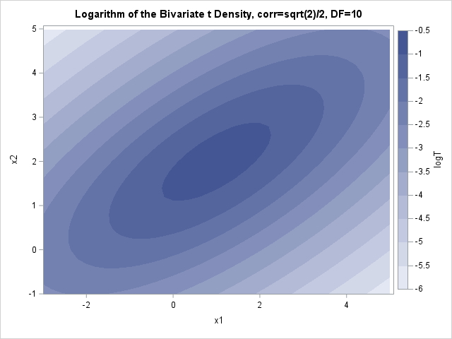
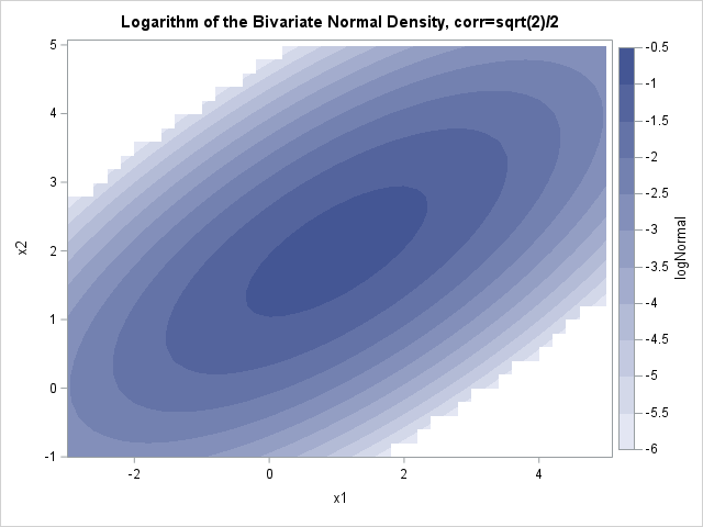
You can see that the ellipses for the normal density are truncated (the jagged edges). For the normal density, the first four ellipses (logNormal > -2) fit entirely within the frame of the graph. The same contours for the t density extend past the frame. Similarly, the contours for log10(Density)= -6 are much smaller for the normal density than for the t density. This is a way to visualize the fact that the normal density approaches 0 exponentially fast as you move away from the center, whereas the t density has a heavier tail with more probability under it.

Summary

This article shows how to implement the PDF function for the t distribution in the SAS/IML language. You can use the PDF to compare the densities of the normal and t distributions. The visualization shows that the normal distribution drops off exponentially fast, so it has "thin" tails. In contrast, the t distribution has fatter tails. Accordingly, random samples from the t distribution tend to have more observations that are far from the center when compared with a random sample from a normal distribution that uses the same parameters.